
Maximum likelihood
Encyclopedia
In statistics, maximum-likelihood estimation (MLE) is a method of estimating
the parameter
s of a statistical model
. When applied to a data set and given a statistical model
, maximum-likelihood estimation provides estimates for the model's parameters.
The method of maximum likelihood corresponds to many well-known estimation methods in statistics. For example, one may be interested in the heights of adult female giraffes, but be unable due to cost or time constraints, to measure the height of every single giraffe in a population. Assuming that the heights are normally (Gaussian) distributed with some unknown mean
and variance
, the mean and variance can be estimated with MLE while only knowing the heights of some sample of the overall population. MLE would accomplish this by taking the mean and variance as parameters and finding particular parametric values that make the observed results the most probable (given the model). In the Kolmogorov structure function
one deals with individual strings. When the models are probability mass functions (required to be computable) then one has a variant of maximum likelihood.
In general, for a fixed set of data and underlying statistical model, the method of maximum likelihood selects values of the model parameters that produce a distribution that gives the observed data the greatest probability (i.e., parameters that maximize the likelihood function
). Maximum-likelihood estimation gives a unified approach to estimation, which is well-defined in the case of the normal distribution and many other problems. However, in some complicated problems, difficulties do occur: in such problems, maximum-likelihood estimators are unsuitable or do not exist.
ƒ0(·). It is however surmised that the function ƒ0 belongs to a certain family of distributions }, called the parametric model
, so that . The value θ0 is unknown and is referred to as the "true value" of the parameter. It is desirable to find some estimator which would be as close to the true value θ0 as possible. Both the observed variables xi and the parameter θ can be vectors.
To use the method of maximum likelihood, one first specifies the joint density function for all observations. For an iid sample this joint density function will be
Estimation theory
Estimation theory is a branch of statistics and signal processing that deals with estimating the values of parameters based on measured/empirical data that has a random component. The parameters describe an underlying physical setting in such a way that their value affects the distribution of the...
the parameter
Parameter
Parameter from Ancient Greek παρά also “para” meaning “beside, subsidiary” and μέτρον also “metron” meaning “measure”, can be interpreted in mathematics, logic, linguistics, environmental science and other disciplines....
s of a statistical model
Statistical model
A statistical model is a formalization of relationships between variables in the form of mathematical equations. A statistical model describes how one or more random variables are related to one or more random variables. The model is statistical as the variables are not deterministically but...
. When applied to a data set and given a statistical model
Statistical model
A statistical model is a formalization of relationships between variables in the form of mathematical equations. A statistical model describes how one or more random variables are related to one or more random variables. The model is statistical as the variables are not deterministically but...
, maximum-likelihood estimation provides estimates for the model's parameters.
The method of maximum likelihood corresponds to many well-known estimation methods in statistics. For example, one may be interested in the heights of adult female giraffes, but be unable due to cost or time constraints, to measure the height of every single giraffe in a population. Assuming that the heights are normally (Gaussian) distributed with some unknown mean
Mean
In statistics, mean has two related meanings:* the arithmetic mean .* the expected value of a random variable, which is also called the population mean....
and variance
Variance
In probability theory and statistics, the variance is a measure of how far a set of numbers is spread out. It is one of several descriptors of a probability distribution, describing how far the numbers lie from the mean . In particular, the variance is one of the moments of a distribution...
, the mean and variance can be estimated with MLE while only knowing the heights of some sample of the overall population. MLE would accomplish this by taking the mean and variance as parameters and finding particular parametric values that make the observed results the most probable (given the model). In the Kolmogorov structure function
Kolmogorov structure function
In 1974 Kolmogorov proposed a non-probabilistic approach to statistics and model selection. Let each data be a finite binary string and models be finite sets of binary strings...
one deals with individual strings. When the models are probability mass functions (required to be computable) then one has a variant of maximum likelihood.
In general, for a fixed set of data and underlying statistical model, the method of maximum likelihood selects values of the model parameters that produce a distribution that gives the observed data the greatest probability (i.e., parameters that maximize the likelihood function
Likelihood function
In statistics, a likelihood function is a function of the parameters of a statistical model, defined as follows: the likelihood of a set of parameter values given some observed outcomes is equal to the probability of those observed outcomes given those parameter values...
). Maximum-likelihood estimation gives a unified approach to estimation, which is well-defined in the case of the normal distribution and many other problems. However, in some complicated problems, difficulties do occur: in such problems, maximum-likelihood estimators are unsuitable or do not exist.
Principles
Suppose there is a sample x1, x2, …, xn of n independent and identically distributed observations, coming from a distribution with an unknown pdfProbability density function
In probability theory, a probability density function , or density of a continuous random variable is a function that describes the relative likelihood for this random variable to occur at a given point. The probability for the random variable to fall within a particular region is given by the...
ƒ0(·). It is however surmised that the function ƒ0 belongs to a certain family of distributions }, called the parametric model
Parametric model
In statistics, a parametric model or parametric family or finite-dimensional model is a family of distributions that can be described using a finite number of parameters...
, so that . The value θ0 is unknown and is referred to as the "true value" of the parameter. It is desirable to find some estimator which would be as close to the true value θ0 as possible. Both the observed variables xi and the parameter θ can be vectors.
To use the method of maximum likelihood, one first specifies the joint density function for all observations. For an iid sample this joint density function will be
-

Now we look at this function from a different perspective by considering the observed values x1, x2, ..., xn to be fixed "parameters" of this function, whereas θ will be the function's variable and allowed to vary freely. From this point of view this distribution function will be called the likelihoodLikelihoodLikelihood is a measure of how likely an event is, and can be expressed in terms of, for example, probability or odds in favor.-Likelihood function:...
:-

In practice it is often more convenient to work with the logarithm of the likelihood function, called the log-likelihood:-

or its scaled version, called the average log-likelihood:-

The hatCircumflexThe circumflex is a diacritic used in the written forms of many languages, and is also commonly used in various romanization and transcription schemes. It received its English name from Latin circumflexus —a translation of the Greek περισπωμένη...
over indicates that it is akin to some estimator. Indeed, estimates the expected log-likelihood of a single observation in the model.
The method of maximum likelihood estimates θ0 by finding a value of θ that maximizes . This method of estimation is a maximum likelihood estimator (MLE) of θ0:-

A MLE estimate is the same regardless of whether we maximize the likelihood or the log-likelihood function, since log is a monotone transformation.
For many models, a maximum likelihood estimator can be found as an explicit function of the observed data x1, …, xn. For many other models, however, no closed-form solution to the maximization problem is known or available, and a MLE has to be found numerically using optimizationOptimization (mathematics)In mathematics, computational science, or management science, mathematical optimization refers to the selection of a best element from some set of available alternatives....
methods. For some problems, there may be multiple estimates that maximize the likelihood. For other problems, no maximum likelihood estimate exists (meaning that the log-likelihood function increases without attaining the supremumSupremumIn mathematics, given a subset S of a totally or partially ordered set T, the supremum of S, if it exists, is the least element of T that is greater than or equal to every element of S. Consequently, the supremum is also referred to as the least upper bound . If the supremum exists, it is unique...
value).
In the exposition above, it is assumed that the data are independent and identically distributed. The method can be applied however to a broader setting, as long as it is possible to write the joint density function , and its parameter θ has a finite dimension which does not depend on the sample size n. In a simpler extension, an allowance can be made for data heterogeneityHomogeneity (statistics)In statistics, homogeneity and its opposite, heterogeneity, arise in describing the properties of a dataset, or several datasets. They relate to the validity of the often convenient assumption that the statistical properties of any one part of an overall dataset are the same as any other part...
, so that the joint density is equal to ƒ1(x1|θ) · ƒ2(x2|θ) · … · ƒn(xn|θ). In the more complicated case of time seriesTime seriesIn statistics, signal processing, econometrics and mathematical finance, a time series is a sequence of data points, measured typically at successive times spaced at uniform time intervals. Examples of time series are the daily closing value of the Dow Jones index or the annual flow volume of the...
models, the independence assumption may have to be dropped as well.
A maximum likelihood estimator coincides with the most probableMaximum a posterioriIn Bayesian statistics, a maximum a posteriori probability estimate is a mode of the posterior distribution. The MAP can be used to obtain a point estimate of an unobserved quantity on the basis of empirical data...
Bayesian estimator given a uniformUniform distribution (continuous)In probability theory and statistics, the continuous uniform distribution or rectangular distribution is a family of probability distributions such that for each member of the family, all intervals of the same length on the distribution's support are equally probable. The support is defined by...
prior distributionPrior probabilityIn Bayesian statistical inference, a prior probability distribution, often called simply the prior, of an uncertain quantity p is the probability distribution that would express one's uncertainty about p before the "data"...
on the parametersParameter spaceIn science, a parameter space is the set of values of parameters encountered in a particular mathematical model. Often the parameters are inputs of a function, in which case the technical term for the parameter space is domain of a function....
.
Properties
Maximum likelihood is the extremum estimatorExtremum estimatorIn statistics and econometrics, extremum estimators is a wide class of estimators for parametric models that are calculated through maximization of a certain objective function, which depends on the data...
obtained by maximizing, as a function of θ, the objective function-

this being the sample analogue of the expected log-likelihood , where this expectation is taken with respect to the true density f(·|θ0).
The maximum-likelihood estimator has essentially no optimalOptimization (mathematics)In mathematics, computational science, or management science, mathematical optimization refers to the selection of a best element from some set of available alternatives....
properties for finite samples. However, the maximum-likelihood estimator possesses a number of attractive asymptotic propertiesAsymptotic theory (statistics)In statistics, asymptotic theory, or large sample theory, is a generic framework for assessment of properties of estimators and statistical tests...
, for many problems; these asymptotic properties include:- Consistency: the estimator converges in probability to the value being estimated.
- Asymptotic normality: as the sample size increases, the distribution of the MLE tends to the Gaussian distribution with mean
 and covariance matrix equal to the inverse of the Fisher informationFisher informationIn mathematical statistics and information theory, the Fisher information is the variance of the score. In Bayesian statistics, the asymptotic distribution of the posterior mode depends on the Fisher information and not on the prior...
matrix. (see e.g. Myung & Navarro 2004). - Efficiency, i.e., it achieves the Cramér–Rao lower bound when the sample size tends to infinity. This means that no asymptotically unbiased estimator has lower asymptotic mean squared errorMean squared errorIn statistics, the mean squared error of an estimator is one of many ways to quantify the difference between values implied by a kernel density estimator and the true values of the quantity being estimated. MSE is a risk function, corresponding to the expected value of the squared error loss or...
than the MLE. - Second-order efficiency after correction for bias.
Consistency
Under the conditions outlined below, the maximum likelihood estimator is consistentConsistent estimatorIn statistics, a sequence of estimators for parameter θ0 is said to be consistent if this sequence converges in probability to θ0...
. The consistency means that having a sufficiently large number of observations n, it is possible to find the value of θ0 with arbitrary precision. In mathematical terms this means that as n goes to infinity the estimator converges in probability to its true value:-

Under slightly stronger conditions, the estimator converges almost surely (or strongly) to:-

To establish consistency, the following conditions are sufficient:
- IdentificationIdentifiabilityIn statistics, identifiability is a property which a model must satisfy in order for inference to be possible. We say that the model is identifiable if it is theoretically possible to learn the true value of this model’s underlying parameter after obtaining an infinite number of observations from it...
of the model:-

In other words, different parameter values θ correspond to different distributions within the model. If this condition did not hold, there would be some value θ1 such that θ0 and θ1 generate an identical distribution of the observable data. Then we wouldn't be able to distinguish between these two parameters even with an infinite amount of data — these parameters would have been observationally equivalentObservational equivalenceIn econometrics, two parameter values are considered observationally equivalent if they both result in the same probability distribution of observable data...
.
The identification condition is absolutely necessary for the ML estimator to be consistent. When this condition holds, the limiting likelihood function ℓ(θ|·) has unique global maximum at θ0.
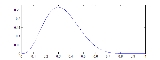
- Compactness: the parameter space Θ of the model is compact.
The identification condition establishes that the log-likelihood has a unique global maximum. Compactness implies that the likelihood cannot approach the maximum value arbitrarily close at some other point (as demonstrated for example in the picture on the right).
Compactness is only a sufficient condition and not a necessary condition. Compactness can be replaced by some other conditions, such as:- both concavityConcave functionIn mathematics, a concave function is the negative of a convex function. A concave function is also synonymously called concave downwards, concave down, convex upwards, convex cap or upper convex.-Definition:...
of the log-likelihood function and compactness of some (nonempty) upper level setLevel setIn mathematics, a level set of a real-valued function f of n variables is a set of the formthat is, a set where the function takes on a given constant value c....
s of the log-likelihood function, or - existence of a compact neighborhood N of θ0 such that outside of N the log-likelihood function is less than the maximum by at least some .
- Continuity: the function ln f(x|θ) is continuous in θ for almost all xs:
-

The continuity here can be replaced with a slightly weaker condition of upper semi-continuity.
- Dominance: there exists an integrable function D(x) such that
-

By the uniform law of large numbers, the dominance condition together with continuity establish the uniform convergence in probability of the log-likelihood: -
- Dominance: there exists an integrable function D(x) such that
- Compactness: the parameter space Θ of the model is compact.
-
The dominance condition can be employed in the case of i.i.d. observations. In the non-i.i.d. case the uniform convergence in probability can be checked by showing that the sequence is stochastically equicontinuousStochastic equicontinuityIn estimation theory in statistics, stochastic equicontinuity is a property of estimators or of estimation procedures that is useful in dealing with their asymptotic behviour as the amount of data increases. It is a version of equicontinuity used in the context of functions of random variables:...
.
If one wants to demonstrate that the ML estimator converges to θ0 almost surely, then a stronger condition of uniform convergence almost surely has to be imposed:-

Asymptotic normality
Maximum-likelihood estimators can lack asymptotic normality and can be inconsistent if there is a failure of one (or more) of the below regularity conditions:
Estimate on boundary. Sometimes the maximum likelihood estimate lies on the boundary of the set of possible parameters, or (if the boundary is not, strictly speaking, allowed) the likelihood gets larger and larger as the parameter approaches the boundary. Standard asymptotic theory needs the assumption that the true parameter value lies away from the boundary. If we have enough data, the maximum likelihood estimate will keep away from the boundary too. But with smaller samples, the estimate can lie on the boundary. In such cases, the asymptotic theory clearly does not give a practically useful approximation. Examples here would be variance-component models, where each component of variance, σ2, must satisfy the constraint σ2 ≥0.
Data boundary parameter-dependent. For the theory to apply in a simple way, the set of data values which has positive probability (or positive probability density) should not depend on the unknown parameter. A simple example where such parameter-dependence does hold is the case of estimating θ from a set of independent identically distributed when the common distribution is uniformUniform distribution (continuous)In probability theory and statistics, the continuous uniform distribution or rectangular distribution is a family of probability distributions such that for each member of the family, all intervals of the same length on the distribution's support are equally probable. The support is defined by...
on the range (0,θ). For estimation purposes the relevant range of θ is such that θ cannot be less than the largest observation. Because the interval (0,θ) is not compactCompact spaceIn mathematics, specifically general topology and metric topology, a compact space is an abstract mathematical space whose topology has the compactness property, which has many important implications not valid in general spaces...
, there exists no maximum for the likelihood function: For any estimate of theta, there exists a greater estimate that also has greater likelihood. In contrast, the interval [0,θ] includes the end-point θ and is compact, in which case the maximum-likelihood estimator exists. However, in this case, the maximum-likelihood estimator is biasedBias of an estimatorIn statistics, bias of an estimator is the difference between this estimator's expected value and the true value of the parameter being estimated. An estimator or decision rule with zero bias is called unbiased. Otherwise the estimator is said to be biased.In ordinary English, the term bias is...
. Asymptotically, this maximum-likelihood estimator is not normally distributed.
Nuisance parameters. For maximum likelihood estimations, a model may have a number of nuisance parameters. For the asymptotic behaviour outlined to hold, the number of nuisance parameters should not increase with the number of observations (the sample size). A well-known example of this case is where observations occur as pairs, where the observations in each pair have a different (unknown) mean but otherwise the observations are independent and Normally distributed with a common variance. Here for 2N observations, there are N+1 parameters. It is well-known that the maximum likelihood estimate for the variance does not converge to the true value of the variance.
Increasing information. For the asymptotics to hold in cases where the assumption of independent identically distributed observations does not hold, a basic requirement is that the amount of information in the data increases indefinitely as the sample size increases. Such a requirement may not be met if either there is too much dependence in the data (for example, if new observations are essentially identical to existing observations), or if new independent observations are subject to an increasing observation error.
Some regularity conditions which ensure this behavior are:- The first and second derivatives of the log-likelihood function must be defined.
- The Fisher information matrix must not be zero, and must be continuous as a function of the parameter.
- The maximum likelihood estimator is consistentConsistent estimatorIn statistics, a sequence of estimators for parameter θ0 is said to be consistent if this sequence converges in probability to θ0...
.
Suppose that conditions for consistency of maximum likelihood estimator are satisfied, and- θ0 ∈ interior(Θ);
- f(x|θ) > 0 and is twice continuously differentiable in θ in some neighborhood N of θ0;
- ∫ supθ∈N||∇θf(x|θ)||dx < ∞, and ∫ supθ∈N||∇θθf(x|θ)||dx < ∞;
- I = E[∇θlnf(x|θ0) ∇θlnf(x|θ0)′] exists and is nonsingular;
- E[ supθ∈N||∇θθlnf(x|θ)||] < ∞.
Then the maximum likelihood estimator has asymptotically normal distribution:-

Proof, skipping the technicalities:
Since the log-likelihood function is differentiable, and θ0 lies in the interior of the parameter set, in the maximum the first-order condition will be satisfied:-

When the log-likelihood is twice differentiable, this expression can be expanded into a Taylor seriesTaylor seriesIn mathematics, a Taylor series is a representation of a function as an infinite sum of terms that are calculated from the values of the function's derivatives at a single point....
around the point :-

where is some point intermediate between θ0 and . From this expression we can derive that-

Here the expression in square brackets converges in probability to H = E[−∇θθln f(x|θ0)] by the law of large numbersLaw of large numbersIn probability theory, the law of large numbers is a theorem that describes the result of performing the same experiment a large number of times...
. The continuous mapping theoremContinuous mapping theoremIn probability theory, the continuous mapping theorem states that continuous functions are limit-preserving even if their arguments are sequences of random variables. A continuous function, in Heine’s definition, is such a function that maps convergent sequences into convergent sequences: if xn → x...
ensures that the inverse of this expression also converges in probability, to H−1. The second sum, by the central limit theoremCentral limit theoremIn probability theory, the central limit theorem states conditions under which the mean of a sufficiently large number of independent random variables, each with finite mean and variance, will be approximately normally distributed. The central limit theorem has a number of variants. In its common...
, converges in distribution to a multivariate normal with mean zero and variance matrix equal to the Fisher informationFisher informationIn mathematical statistics and information theory, the Fisher information is the variance of the score. In Bayesian statistics, the asymptotic distribution of the posterior mode depends on the Fisher information and not on the prior...
I. Thus, applying the Slutsky's theoremSlutsky's theoremIn probability theory, Slutsky’s theorem extends some properties of algebraic operations on convergent sequences of real numbers to sequences of random variables.The theorem was named after Eugen Slutsky. Slutsky’s theorem is also attributed to Harald Cramér....
to the whole expression, we obtain that-

Finally, the information equality guarantees that when the model is correctly specified, matrix H will be equal to the Fisher information I, so that the variance expression simplifies to just I−1.
Functional invariance
The maximum likelihood estimator selects the parameter value which gives the observed data the largest possible probability (or probability density, in the continuous case). If the parameter consists of a number of components, then we define their separate maximum likelihood estimators, as the corresponding component of the MLE of the complete parameter. Consistent with this, if is the MLE for θ, and if g(θ) is any transformation of θ, then the MLE for α = g(θ) is by definition

It maximizes the so-called profile likelihood:
The MLE is also invariant with respect to certain transformations of the data. If Y = g(X) where g is one to one and does not depend on the parameters to be estimated, then the density functions satisfy
and hence the likelihood functions for X and Y differ only by a factor that does not depend on the model parameters.
For example, the MLE parameters of the log-normal distribution are the same as those of the normal distribution fitted to the logarithm of the data.
Higher-order properties
The standard asymptotics tells that the maximum-likelihood estimator is √n-consistent and asymptotically efficient, meaning that it reaches the Cramér–Rao bound:-

where I is the Fisher information matrix:-

In particular, it means that the biasBias of an estimatorIn statistics, bias of an estimator is the difference between this estimator's expected value and the true value of the parameter being estimated. An estimator or decision rule with zero bias is called unbiased. Otherwise the estimator is said to be biased.In ordinary English, the term bias is...
of the maximum-likelihood estimator is equal to zero up to the order n−1/2. However when we consider the higher-order terms in the expansion of the distribution of this estimator, it turns out that θmle has bias of order n−1. This bias is equal to (componentwise)-

where Einstein's summation conventionEinstein notationIn mathematics, especially in applications of linear algebra to physics, the Einstein notation or Einstein summation convention is a notational convention useful when dealing with coordinate formulae...
over the repeating indices has been adopted; I jk denotes the j,k-th component of the inverse Fisher information matrix I−1, and-

Using these formulas it is possible to estimate the second-order bias of the maximum likelihood estimator, and correct for that bias by subtracting it:-

This estimator is unbiased up to the terms of order n−1, and is called the bias-corrected maximum likelihood estimator.
This bias-corrected estimator is second-order efficient (at least within the curved exponential family), meaning that it has minimal mean squared error among all second-order bias-corrected estimators, up to the terms of the order n−2. It is possible to continue this process, that is to derive the third-order bias-correction term, and so on. However as was shown by , the maximum-likelihood estimator is not third-order efficient.
Least Squares as Maximum Likelihood Estimator
Suppose that we are given a data set of n points (xi,yi) for i=1,...,n and we are to estimate m parameters for i=1,...,m. The model gives y(x) as a function of
  :
:
-

One can do the Least-Squares fitLeast squaresThe method of least squares is a standard approach to the approximate solution of overdetermined systems, i.e., sets of equations in which there are more equations than unknowns. "Least squares" means that the overall solution minimizes the sum of the squares of the errors made in solving every...
to minimize over
over  . This can be justified using Bayesian probabilityBayesian probabilityBayesian probability is one of the different interpretations of the concept of probability and belongs to the category of evidential probabilities. The Bayesian interpretation of probability can be seen as an extension of logic that enables reasoning with propositions, whose truth or falsity is...
as follows:
Suppose each data point has an error uniformly and randomly (iidIndependent and identically distributed random variablesIn probability theory and statistics, a sequence or other collection of random variables is independent and identically distributed if each random variable has the same probability distribution as the others and all are mutually independent....
) distributed with Normal distribution around the "actual" model y(x) and suppose that is the standard deviation of the error at point xi. Then the probability of the dataset is the product of probabilities at each point :
-

One can then invoke Bayes' theoremBayes' theoremIn probability theory and applications, Bayes' theorem relates the conditional probabilities P and P. It is commonly used in science and engineering. The theorem is named for Thomas Bayes ....
and get,
Where, is the prior probability distribution over all the models. This is often taken as constant (noninformative prior).
One can then seek to maximize or minimize the negative logarithm of the same which is equivalent to minimizing the least squares sum.
Discrete uniform distribution
Consider a case where n tickets numbered from 1 to n are placed in a box and one is selected at random (see uniform distribution); thus, the sample size is 1. If n is unknown, then the maximum-likelihood estimator of n is the number m on the drawn ticket. (The likelihood is 0 for n < m, 1/n for n ≥ m, and this is greatest when n = m. Note that the maximum likelihood estimate of n occurs at the lower extreme of possible values {m, m + 1, ...}, rather than somewhere in the "middle" of the range of possible values, which would result in less bias.) The expected valueExpected valueIn probability theory, the expected value of a random variable is the weighted average of all possible values that this random variable can take on...
of the number m on the drawn ticket, and therefore the expected value of , is (n + 1)/2. As a result, the maximum likelihood estimator for n will systematically underestimate n by (n − 1)/2 with a sample size of 1.
Discrete distribution, finite parameter space
Suppose one wishes to determine just how biased an unfair coin is. Call the probability of tossing a HEAD p. The goal then becomes to determine p.
Suppose the coin is tossed 80 times: i.e., the sample might be something like x1 = H, x2 = T, ..., x80 = T, and the count of the number of HEADS "H" is observed.
The probability of tossing TAILS is 1 − p (so here p is θ above). Suppose the outcome is 49 HEADS and 31 TAILS, and suppose the coin was taken from a box containing three coins: one which gives HEADS with probability p = 1/3, one which gives HEADS with probability p = 1/2 and another which gives HEADS with probability p = 2/3. The coins have lost their labels, so which one it was is unknown. Using maximum likelihood estimation the coin that has the largest likelihood can be found, given the data that were observed. By using the probability mass functionProbability mass functionIn probability theory and statistics, a probability mass function is a function that gives the probability that a discrete random variable is exactly equal to some value...
of the binomial distribution with sample size equal to 80, number successes equal to 49 but different values of p (the "probability of success"), the likelihood function (defined below) takes one of three values:
The likelihood is maximized when p = 2/3, and so this is the maximum likelihood estimate for p.
Discrete distribution, continuous parameter space
Now suppose that there was only one coin but its p could have been any value 0 ≤ p ≤ 1. The likelihood function to be maximised is
and the maximisation is over all possible values 0 ≤ p ≤ 1.
One way to maximize this function is by differentiatingDerivativeIn calculus, a branch of mathematics, the derivative is a measure of how a function changes as its input changes. Loosely speaking, a derivative can be thought of as how much one quantity is changing in response to changes in some other quantity; for example, the derivative of the position of a...
with respect to p and setting to zero:
which has solutions p = 0, p = 1, and p = 49/80. The solution which maximizes the likelihood is clearly p = 49/80 (since p = 0 and p = 1 result in a likelihood of zero). Thus the maximum likelihood estimator for p is 49/80.
This result is easily generalized by substituting a letter such as t in the place of 49 to represent the observed number of 'successes' of our Bernoulli trialBernoulli trialIn the theory of probability and statistics, a Bernoulli trial is an experiment whose outcome is random and can be either of two possible outcomes, "success" and "failure"....
s, and a letter such as n in the place of 80 to represent the number of Bernoulli trials. Exactly the same calculation yields the maximum likelihood estimator t / n for any sequence of n Bernoulli trials resulting in t 'successes'.
Continuous distribution, continuous parameter space
For the normal distribution which has probability density functionProbability density functionIn probability theory, a probability density function , or density of a continuous random variable is a function that describes the relative likelihood for this random variable to occur at a given point. The probability for the random variable to fall within a particular region is given by the...
the corresponding probability density functionProbability density functionIn probability theory, a probability density function , or density of a continuous random variable is a function that describes the relative likelihood for this random variable to occur at a given point. The probability for the random variable to fall within a particular region is given by the...
for a sample of n independent identically distributed normal random variables (the likelihood) is

or more conveniently:

where is the sample mean.
This family of distributions has two parameters: θ = (μ, σ), so we maximize the likelihood, , over both parameters simultaneously, or if possible, individually.
Since the logarithmNatural logarithmThe natural logarithm is the logarithm to the base e, where e is an irrational and transcendental constant approximately equal to 2.718281828...
is a continuousContinuous functionIn mathematics, a continuous function is a function for which, intuitively, "small" changes in the input result in "small" changes in the output. Otherwise, a function is said to be "discontinuous". A continuous function with a continuous inverse function is called "bicontinuous".Continuity of...
strictly increasing function over the rangeRange (mathematics)In mathematics, the range of a function refers to either the codomain or the image of the function, depending upon usage. This ambiguity is illustrated by the function f that maps real numbers to real numbers with f = x^2. Some books say that range of this function is its codomain, the set of all...
of the likelihood, the values which maximize the likelihood will also maximize its logarithm. Since maximizing the logarithm often requires simpler algebra, it is the logarithm which is maximized below. (Note: the log-likelihood is closely related to information entropyInformation entropyIn information theory, entropy is a measure of the uncertainty associated with a random variable. In this context, the term usually refers to the Shannon entropy, which quantifies the expected value of the information contained in a message, usually in units such as bits...
and Fisher informationFisher informationIn mathematical statistics and information theory, the Fisher information is the variance of the score. In Bayesian statistics, the asymptotic distribution of the posterior mode depends on the Fisher information and not on the prior...
.)
which is solved by
This is indeed the maximum of the function since it is the only turning point in μ and the second derivative is strictly less than zero. Its expectation value is equal to the parameter μ of the given distribution,

which means that the maximum-likelihood estimator is unbiased.
Similarly we differentiate the log likelihood with respect to σ and equate to zero:
which is solved by
Inserting we obtain

To calculate its expected value, it is convenient to rewrite the expression in terms of zero-mean random variables (statistical error) . Expressing the estimate in these variables yields

Simplifying the expression above, utilizing the facts that and
and  , allows us to obtain

This means that the estimator is biased. However,
  is consistent.
Formally we say that the maximum likelihood estimator for is:
is:

In this case the MLEs could be obtained individually. In general this may not be the case, and the MLEs would have to be obtained simultaneously.
Non-independent variables
It may be the case that variables are correlated, that is, not independent. Two random variables X and Y are independent only if their joint probability density function is the product of the individual probability density functions, i.e.
Suppose one constructs an order-n Gaussian vector out of random variables , where each variable has means given by
  . Furthermore, let the covariance matrixCovariance matrixIn probability theory and statistics, a covariance matrix is a matrix whose element in the i, j position is the covariance between the i th and j th elements of a random vector...
be denoted by
The joint probability density function of these n random variables is then given by:

In the two variable case, the joint probability density function is given by:

In this and other cases where a joint density function exists, the likelihood function is defined as above, under Principles, using this density.
Applications
Maximum likelihood estimation is used for a wide range of statistical models, including:- linear modelLinear modelIn statistics, the term linear model is used in different ways according to the context. The most common occurrence is in connection with regression models and the term is often taken as synonymous with linear regression model. However the term is also used in time series analysis with a different...
s and generalized linear modelGeneralized linear modelIn statistics, the generalized linear model is a flexible generalization of ordinary linear regression. The GLM generalizes linear regression by allowing the linear model to be related to the response variable via a link function and by allowing the magnitude of the variance of each measurement to...
s; - exploratoryFactor analysisFactor analysis is a statistical method used to describe variability among observed, correlated variables in terms of a potentially lower number of unobserved, uncorrelated variables called factors. In other words, it is possible, for example, that variations in three or four observed variables...
and confirmatory factor analysisConfirmatory factor analysisIn statistics, confirmatory factor analysis is a special form of factor analysis. It is used to test whether measures of a construct are consistent with a researcher's understanding of the nature of that construct . In contrast to exploratory factor analysis, where all loadings are free to vary,...
; - structural equation modelingStructural equation modelingStructural equation modeling is a statistical technique for testing and estimating causal relations using a combination of statistical data and qualitative causal assumptions...
; - many situations in the context of hypothesis testing and confidence intervalConfidence intervalIn statistics, a confidence interval is a particular kind of interval estimate of a population parameter and is used to indicate the reliability of an estimate. It is an observed interval , in principle different from sample to sample, that frequently includes the parameter of interest, if the...
formation; - discrete choiceDiscrete choiceIn economics, discrete choice problems involve choices between two or more discrete alternatives, such as entering or not entering the labor market, or choosing between modes of transport. Such choices contrast with standard consumption models in which the quantity of each good consumed is assumed...
models.
These uses arise across applications in widespread set of fields, including:- communication systems;
- psychometricsPsychometricsPsychometrics is the field of study concerned with the theory and technique of psychological measurement, which includes the measurement of knowledge, abilities, attitudes, personality traits, and educational measurement...
; - econometricsEconometricsEconometrics has been defined as "the application of mathematics and statistical methods to economic data" and described as the branch of economics "that aims to give empirical content to economic relations." More precisely, it is "the quantitative analysis of actual economic phenomena based on...
; - time-delay of arrival (TDOA) in acoustic or electromagnetic detection;
- data modeling in nuclear and particle physics;
- magnetic resonance imaging;
- computational phylogeneticsComputational phylogeneticsComputational phylogenetics is the application of computational algorithms, methods and programs to phylogenetic analyses. The goal is to assemble a phylogenetic tree representing a hypothesis about the evolutionary ancestry of a set of genes, species, or other taxa...
; - origin/destination and path-choice modeling in transport networks.
History
Maximum-likelihood estimation was recommended, analyzed (with flawed attempts at proofMathematical proofIn mathematics, a proof is a convincing demonstration that some mathematical statement is necessarily true. Proofs are obtained from deductive reasoning, rather than from inductive or empirical arguments. That is, a proof must demonstrate that a statement is true in all cases, without a single...
s) and vastly popularized by R. A. FisherRonald FisherSir Ronald Aylmer Fisher FRS was an English statistician, evolutionary biologist, eugenicist and geneticist. Among other things, Fisher is well known for his contributions to statistics by creating Fisher's exact test and Fisher's equation...
between 1912 and 1922 (although it had been used earlier by GaussGaussGauss may refer to:*Carl Friedrich Gauss, German mathematician and physicist*Gauss , a unit of magnetic flux density or magnetic induction*GAUSS , a software package*Gauss , a crater on the moon...
, Laplace, ThieleThorvald N. ThieleThorvald Nicolai Thiele was a Danish astronomer, actuary and mathematician, most notable for his work in statistics, interpolation and the three-body problem. He was the first to propose a mathematical theory of Brownian motion...
, and F. Y. EdgeworthFrancis Ysidro EdgeworthFrancis Ysidro Edgeworth FBA was an Irish philosopher and political economist who made significant contributions to the methods of statistics during the 1880s...
). Reviews of the development of maximum likelihood have been provided by a number of authors.
Much of the theory of maximum-likelihood estimation was first developed for Bayesian statisticsBayesian statisticsBayesian statistics is that subset of the entire field of statistics in which the evidence about the true state of the world is expressed in terms of degrees of belief or, more specifically, Bayesian probabilities...
, and then simplified by later authors.
See also
- Other estimation methods
- Restricted maximum likelihoodRestricted maximum likelihoodIn statistics, the restricted maximum likelihood approach is a particular form of maximum likelihood estimation which does not base estimates on a maximum likelihood fit of all the information, but instead uses a likelihood function calculated from a transformed set of data, so that nuisance...
, a variation using a likelihood function calculated from a transformed set of data. - Quasi-maximum likelihoodQuasi-maximum likelihoodA quasi-maximum likelihood estimate is an estimate of a parameter θ in a statistical model that is formed by maximizing a function that is related to the logarithm of the likelihood function, but is not equal to it...
estimator, a MLE estimator that is misspecified, but still consistent. - Maximum a posteriori (MAP) estimatorMaximum a posterioriIn Bayesian statistics, a maximum a posteriori probability estimate is a mode of the posterior distribution. The MAP can be used to obtain a point estimate of an unobserved quantity on the basis of empirical data...
, for a contrast in the way to calculate estimators when prior knowledge is postulated. - Method of supportMethod of supportIn statistics, the method of support is a technique that is used to make inferences from datasets.According to A. W. F. Edwards, the method of support aims to make inferences about unknown parameters in terms of the relative support, or log likelihood, induced by a set of data for a particular...
, a variation of the maximum likelihood technique. - M-estimatorM-estimatorIn statistics, M-estimators are a broad class of estimators, which are obtained as the minima of sums of functions of the data. Least-squares estimators and many maximum-likelihood estimators are M-estimators. The definition of M-estimators was motivated by robust statistics, which contributed new...
, an approach used in robust statistics. - Method of moments (statistics), another popular method for finding parameters of distributions.
- Generalized method of momentsGeneralized method of momentsIn econometrics, generalized method of moments is a generic method for estimating parameters in statistical models. Usually it is applied in the context of semiparametric models, where the parameter of interest is finite-dimensional, whereas the full shape of the distribution function of the data...
are methods related to the likelihood equation in maximum likelihood estimation. - Minimum distance estimationMinimum distance estimationMinimum distance estimation is a statistical method for fitting a mathematical model to data, usually the empirical distribution.-Definition:...
- Maximum spacing estimationMaximum spacing estimationIn statistics, maximum spacing estimation , or maximum product of spacing estimation , is a method for estimating the parameters of a univariate statistical model...
, a related method that is more robust in many situations.
- Restricted maximum likelihood
- Related concepts:
- Fisher informationFisher informationIn mathematical statistics and information theory, the Fisher information is the variance of the score. In Bayesian statistics, the asymptotic distribution of the posterior mode depends on the Fisher information and not on the prior...
, information matrix, its relationship to covariance matrix of ML estimates - Likelihood functionLikelihood functionIn statistics, a likelihood function is a function of the parameters of a statistical model, defined as follows: the likelihood of a set of parameter values given some observed outcomes is equal to the probability of those observed outcomes given those parameter values...
, a description on what likelihood functions are. - Mean squared errorMean squared errorIn statistics, the mean squared error of an estimator is one of many ways to quantify the difference between values implied by a kernel density estimator and the true values of the quantity being estimated. MSE is a risk function, corresponding to the expected value of the squared error loss or...
, a measure of how 'good' an estimator of a distributional parameter is (be it the maximum likelihood estimator or some other estimator). - Extremum estimatorExtremum estimatorIn statistics and econometrics, extremum estimators is a wide class of estimators for parametric models that are calculated through maximization of a certain objective function, which depends on the data...
, a more general class of estimators to which MLE belongs. - The Rao–Blackwell theoremRao–Blackwell theoremIn statistics, the Rao–Blackwell theorem, sometimes referred to as the Rao–Blackwell–Kolmogorov theorem, is a result which characterizes the transformation of an arbitrarily crude estimator into an estimator that is optimal by the mean-squared-error criterion or any of a variety of similar...
, a result which yields a process for finding the best possible unbiased estimator (in the sense of having minimal mean squared errorMean squared errorIn statistics, the mean squared error of an estimator is one of many ways to quantify the difference between values implied by a kernel density estimator and the true values of the quantity being estimated. MSE is a risk function, corresponding to the expected value of the squared error loss or...
). The MLE is often a good starting place for the process. - Sufficient statistic, a function of the data through which the MLE (if it exists and is unique) will depend on the data.
- The BHHH algorithm is a non-linear optimization algorithm that is popular for Maximum Likelihood estimations.
- Fisher information
External links
- linear model
-
-
-
-
-
-
-
-
-
-
-
- Identification
-
-
-
-
-
-
