
Computational fluid dynamics
Encyclopedia
Computational fluid dynamics, usually abbreviated as CFD, is a branch of fluid mechanics
that uses numerical methods and algorithms to solve and analyze problems that involve fluid flows. Computers are used to perform the calculations required to simulate the interaction of liquids and gases with surfaces defined by boundary conditions. With high-speed supercomputer
s, better solutions can be achieved. Ongoing research yields software that improves the accuracy and speed of complex simulation scenarios such as transonic or turbulent
flows. Initial validation of such software is performed using a wind tunnel
with the final validation coming in flight test
s.
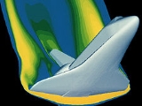
_mach_7_computational_fluid_dynamic_(cfd).jpg) The fundamental basis of almost all CFD problems are the Navier–Stokes equations, which define any single-phase fluid flow. These equations can be simplified by removing terms describing viscosity to yield the Euler equations. Further simplification, by removing terms describing vorticity yields the full potential equations. Finally, these equations can be linearized to yield the linearized potential equations.
The fundamental basis of almost all CFD problems are the Navier–Stokes equations, which define any single-phase fluid flow. These equations can be simplified by removing terms describing viscosity to yield the Euler equations. Further simplification, by removing terms describing vorticity yields the full potential equations. Finally, these equations can be linearized to yield the linearized potential equations.
Historically, methods were first developed to solve the Linearized Potential equations. Two-dimensional methods, using conformal transformations of the flow about a cylinder
to the flow about an airfoil
were developed in the 1930s. The computer power available paced development of three-dimensional
methods. The first paper on a practical three-dimensional method to solve the linearized potential equations was published by John Hess and A.M.O. Smith of Douglas Aircraft in 1967. This method discretized the surface of the geometry with panels, giving rise to this class of programs being called Panel Methods. Their method itself was simplified, in that it did not include lifting flows and hence was mainly applied to ship hulls and aircraft fuselages. The first lifting Panel Code (A230) was described in a paper written by Paul Rubbert and Gary Saaris of Boeing Aircraft in 1968. In time, more advanced three-dimensional Panel Codes were developed at Boeing
(PANAIR, A502), Lockheed
(Quadpan), Douglas
(HESS), McDonnell Aircraft
(MACAERO), NASA
(PMARC) and Analytical Methods (WBAERO, USAERO and VSAERO). Some (PANAIR, HESS and MACAERO) were higher order codes, using higher order distributions of surface singularities, while others (Quadpan, PMARC, USAERO and VSAERO) used single singularities on each surface panel. The advantage of the lower order codes was that they ran much faster on the computers of the time. Today, VSAERO has grown to be a multi-order code and is the most widely used program of this class. It has been used in the development of many submarine
s, surface ship
s, automobile
s, helicopter
s , aircraft
, and more recently wind turbines. Its sister code, USAERO is an unsteady panel method that has also been used for modeling such things as high speed trains and racing yacht
s. The NASA PMARC code from an early version of VSAERO and a derivative of PMARC, named CMARC, is also commercially available.
In the two-dimensional realm, a number of Panel Codes have been developed for airfoil analysis and design. The codes typically have a boundary layer
analysis included, so that viscous effects can be modeled. Professor Richard Eppler of the University of Stuttgart
developed the PROFIL
code, partly with NASA funding, which became available in the early 1980s. This was soon followed by MIT Professor Mark Drela's XFOIL
code. Both PROFIL and XFOIL incorporate two-dimensional panel codes, with coupled boundary layer codes for airfoil analysis work. PROFIL uses a conformal transformation method for inverse airfoil design, while XFOIL has both a conformal transformation and an inverse panel method for airfoil design. Both codes are used.
An intermediate step between Panel Codes and Full Potential codes were codes that used the Transonic Small Disturbance equations. In particular, the three-dimensional WIBCO code, developed by Charlie Boppe of Grumman Aircraft in the early 1980s has seen heavy use.
Developers turned to Full Potential codes, as panel methods could not calculate the non-linear flow present at transonic
speeds. The first description of a means of using the Full Potential equations was published by Earll Murman and Julian Cole
of Boeing in 1970. Frances Bauer, Paul Garabedian
and David Korn of the Courant Institute at New York University
(NYU) wrote a series of two-dimensional Full Potential airfoil codes that were widely used, the most important being named Program H. A further growth of Program H was developed by Bob Melnik and his group at Grumman Aerospace as Grumfoil. Antony Jameson
, originally at Grumman Aircraft and the Courant Institute of NYU, worked with David Caughey to develop the important three-dimensional Full Potential code FLO22 in 1975. Many Full Potential codes emerged after this, culminating in Boeing's Tranair (A633) code, which still sees heavy use.
The next step was the Euler equations, which promised to provide more accurate solutions of transonic flows. The methodology used by Jameson in his three-dimensional FLO57 code (1981) was used by others to produce such programs as Lockheed's TEAM program and IAI/Analytical Methods' MGAERO program. MGAERO is unique in being a structured cartesian
mesh code, while most other such codes use structured body-fitted grids (with the exception of NASA's highly successful CART3D code, Lockheed's SPLITFLOW code and Georgia Tech
's NASCART-GT). Antony Jameson
also developed the three-dimensional AIRPLANE code (1985) which made use of unstructured tetrahedral grids.
In the two-dimensional realm, Mark Drela and Michael Giles, then graduate students at MIT, developed the ISES Euler program (actually a suite of programs) for airfoil design and analysis. This code first became available in 1986 and has been further developed to design, analyze and optimize single or multi-element airfoils, as the MSES program. MSES sees wide use throughout the world. A derivative of MSES, for the design and analysis of airfoils in a cascade, is MISES, developed by Harold "Guppy" Youngren while he was a graduate student at MIT.
The Navier–Stokes equations were the ultimate target of developers. Two-dimensional codes, such as NASA Ames' ARC2D code first emerged. A number of three-dimensional codes were developed (ARC3D, OVERFLOW
, CFL3D are three successful NASA contributions), leading to numerous commercial packages.
Some of the discretization methods being used are:

where is the vector of conserved variables,
  is the vector of fluxes (see Euler equations or Navier–Stokes equations),
  is the volume of the control volume element, and
  is the surface area of the control volume element.
In this method, a weighted residual equation is formed:

where is the equation residual at an element vertex
  ,
,  is the conservation equation expressed on an element basis,
  is the weight factor, and
  is the volume of the element.

where is the vector of conserved variables, and
  ,
,  , and
, and  are the fluxes in the
  ,
,  , and
, and  directions respectively.
 . In a spectral element method however, the interpolating and test functions are chosen to be polynomials of a very high order (typically e.g. of the 10th order in CFD applications). This guarantees the rapid convergence of the method. Furthermore, very efficient integration procedures must be used, since the number of integrations to be performed in a numerical codes is big. Thus, high order Gauss integration quadratures are employed, since they achieve the highest accuracy with the smallest number of computations to be carried out.
At the time there are some academic CFD codes based on the spectral element method and some more are currently under development, since the new time-stepping schemes arrise in the scientific world. You can refer to the C-CFD website to see movies of incompressible flows in channels simulated with a spectral element solver or to the Numerical Mechanics (see bottom of the page) website to see a movie of the lid-driven cavity flow obtained with a compeletely novel unconditionally stable time-stepping scheme combined with a spectral element solver.
.
The chief difficulty in modeling turbulent flows comes from the wide range of length and time scales associated with turbulent flow. As a result, turbulence models can be classified based on the range of these length and time scales that are modeled and the range of length and time scales that are resolved. The more turbulent scales that are resolved, the finer the resolution of the simulation, and therefore the higher the computational cost. If a majority or all of the turbulent scales are modeled, the computational cost is very low, but the tradeoff comes in the form of decreased accuracy.
In addition to the wide range of length and time scales and the associated computational cost, the governing equations of fluid dynamics contain a non-linear convection term and a non-linear and non-local pressure gradient term. These nonlinear equations must be solved numerically with the appropriate boundary and initial conditions.
. This adds a second order tensor of unknowns for which various models can provide different levels of closure. It is a common misconception that the RANS equations do not apply to flows with a time-varying mean flow because these equations are 'time-averaged'. In fact, statistically unsteady (or non-stationary) flows can equally be treated. This is sometimes referred to as URANS. There is nothing inherent in Reynolds averaging to preclude this, but the turbulence models used to close the equations are valid only as long as the time over which these changes in the mean occur is large compared to the time scales of the turbulent motion containing most of the energy.
RANS models can be divided into two broad approaches:
Boussinesq hypothesis
: This method involves using an algebraic equation for the Reynolds stresses which include determining the turbulent viscosity, and depending on the level of sophistication of the model, solving transport equations for determining the turbulent kinetic energy and dissipation. Models include k-ε (Launder
and Spalding
), Mixing Length Model (Prandtl), and Zero Equation Model (Cebeci and Smith). The models available in this approach are often referred to by the number of transport equations associated with the method. For example, the Mixing Length model is a "Zero Equation" model because no transport equations are solved; the is a "Two Equation" model because two transport equations (one for
  and one for
  ) are solved.
Reynolds stress model (RSM): This approach attempts to actually solve transport equations for the Reynolds stresses. This means introduction of several transport equations for all the Reynolds stresses and hence this approach is much more costly in CPU effort.
(LES) is a technique in which the smallest scales of the flow are removed through a filtering operation, and their effect modeled using subgrid scale models. This allows the largest and most important scales of the turbulence to be resolved, while greatly reducing the computational cost incurred by the smallest scales. This method requires greater computational resources than RANS methods, but is far cheaper than DNS.
s (DES) is a modification of a RANS model in which the model switches to a subgrid scale formulation in regions fine enough for LES calculations. Regions near solid boundaries and where the turbulent length scale is less than the maximum grid dimension are assigned the RANS mode of solution. As the turbulent length scale exceeds the grid dimension, the regions are solved using the LES mode. Therefore the grid resolution for DES is not as demanding as pure LES, thereby considerably cutting down the cost of the computation. Though DES was initially formulated for the Spalart-Allmaras model (Spalart et al., 1997), it can be implemented with other RANS models (Strelets, 2001), by appropriately modifying the length scale which is explicitly or implicitly involved in the RANS model. So while Spalart-Allmaras model based DES acts as LES with a wall model, DES based on other models (like two equation models) behave as a hybrid RANS-LES model. Grid generation is more complicated than for a simple RANS or LES case due to the RANS-LES switch. DES is a non-zonal approach and provides a single smooth velocity field across the RANS and the LES regions of the solutions.
(DNS) resolves the entire range of turbulent length scales. This marginalizes the effect of models, but is extremely expensive. The computational cost is proportional to . DNS is intractable for flows with complex geometries or flow configurations.
filtering. The approach has much in common with LES, since it uses decomposition and resolves only the filtered portion, but different in that it does not use a linear, low-pass filter. Instead, the filtering operation is based on wavelets, and the filter can be adapted as the flow field evolves. Farge and Schneider tested the CVS method with two flow configurations and showed that the coherent portion of the flow exhibited the energy spectrum exhibited by the total flow, and corresponded to coherent structures (vortex tubes
), while the incoherent parts of the flow composed homogeneous background noise, which exhibited no organized structures. Goldstein and Oleg applied the CVS model to large eddy simulation, but did not assume that the wavelet filter completely eliminated all coherent motions from the subfilter scales. By employing both LES and CVS filtering, they showed that the SFS dissipation was dominated by the SFS flow field's coherent portion.
(PDF) methods for turbulence, first introduced by Lundgren
, are based on tracking the one-point PDF of the velocity, , which gives the probability of the velocity at point
  being between
  and
and  . This approach is analogous to the kinetic theory
of gases, in which the macroscopic properties of a gas are described by a large number of particles. PDF methods are unique in that they can be applied in the framework of a number of different turbulence models; the main differences occur in the form of the PDF transport equation. For example, in the context of large eddy simulation
, the PDF becomes the filtered PDF. PDF methods can also be used to describe chemical reactions, and are particularly useful for simulating chemically reacting flows because the chemical source term is closed and does not require a model. The PDF is commonly tracked by using Lagrangian particle methods; when combined with large eddy simulation, this leads to a Langevin equation
for subfiler particle evolution.
(in which the motion of N objects is tied to their mutual influences). A breakthrough came in the late 1980s with the development of the fast multipole method
(FMM), an algorithm by V. Rokhlin (Yale) and L. Greengard (Courant Institute). This breakthrough paved the way to practical computation of the velocities from the vortex elements and is the basis of successful algorithms. They are especially well-suited to simulating filamentary motion, such as wisps of smoke, in real-time simulations such as video games, because of the fine detail achieved using minimal computation.
Software based on the vortex method offer a new means for solving tough fluid dynamics problems with minimal user intervention. All that is required is specification of problem geometry and setting of boundary and initial conditions. Among the significant advantages of this modern technology;
(VC) method is an Eulerian technique used in the simulation of turbulent wakes. It uses a solitary-wave like approach to produce a stable solution with no numerical spreading. VC can capture the small scale features to within as few as 2 grid cells. Within these features, a nonlinear difference equation is solved as opposed to the finite difference equation. VC is similar to shock capturing methods
, where conservation laws are satisfied, so that the essential integral quantities are accurately computed.
has received a lot of attention lately, for problems that do not have dispersed particles, but the Level set method
and front tracking are also valuable approaches . Most of these methods are either good in maintaining a sharp interface or at conserving mass . This is crucial since the evaluation of the density, viscosity and surface tension is based on the values averaged over the interface. Lagrangian multiphase models, which are used for dispersed media, are based on solving the Lagrangian equation of motion for the dispersed phase.
or Krylov subspace
methods. Krylov methods such as GMRES
, typically used with preconditioning
, operate by minimizing the residual over successive subspaces generated by the preconditioned operator.
Multigrid
has the advantage of asymptotically optimal performance on many problems. Traditional solvers and preconditioners are effective at reducing high-frequency components of the residual, but low-frequency components typically require many iterations to reduce. By operating on multiple scales, multigrid reduces all components of the residual by similar factors, leading to a mesh-independent number of iterations.
For indefinite systems, preconditioners such as incomplete LU factorization
, additive Schwarz, and multigrid
perform poorly or fail entirely, so the problem structure must be used for effective preconditioning. Methods commonly used in CFD are the SIMPLE
and Uzawa algorithms which exhibit mesh-dependent convergence rates, but recent advances based on block LU factorization combined with multigrid for the resulting definite systems have led to preconditioners that deliver mesh-independent convergence rates.
Fluid mechanics
Fluid mechanics is the study of fluids and the forces on them. Fluid mechanics can be divided into fluid statics, the study of fluids at rest; fluid kinematics, the study of fluids in motion; and fluid dynamics, the study of the effect of forces on fluid motion...
that uses numerical methods and algorithms to solve and analyze problems that involve fluid flows. Computers are used to perform the calculations required to simulate the interaction of liquids and gases with surfaces defined by boundary conditions. With high-speed supercomputer
Supercomputer
A supercomputer is a computer at the frontline of current processing capacity, particularly speed of calculation.Supercomputers are used for highly calculation-intensive tasks such as problems including quantum physics, weather forecasting, climate research, molecular modeling A supercomputer is a...
s, better solutions can be achieved. Ongoing research yields software that improves the accuracy and speed of complex simulation scenarios such as transonic or turbulent
Turbulence
In fluid dynamics, turbulence or turbulent flow is a flow regime characterized by chaotic and stochastic property changes. This includes low momentum diffusion, high momentum convection, and rapid variation of pressure and velocity in space and time...
flows. Initial validation of such software is performed using a wind tunnel
Wind tunnel
A wind tunnel is a research tool used in aerodynamic research to study the effects of air moving past solid objects.-Theory of operation:Wind tunnels were first proposed as a means of studying vehicles in free flight...
with the final validation coming in flight test
Flight test
Flight test is a branch of aeronautical engineering that develops and gathers data during flight of an aircraft and then analyzes the data to evaluate the flight characteristics of the aircraft and validate its design, including safety aspects...
s.
Background and history
Historically, methods were first developed to solve the Linearized Potential equations. Two-dimensional methods, using conformal transformations of the flow about a cylinder
Cylinder (geometry)
A cylinder is one of the most basic curvilinear geometric shapes, the surface formed by the points at a fixed distance from a given line segment, the axis of the cylinder. The solid enclosed by this surface and by two planes perpendicular to the axis is also called a cylinder...
to the flow about an airfoil
Airfoil
An airfoil or aerofoil is the shape of a wing or blade or sail as seen in cross-section....
were developed in the 1930s. The computer power available paced development of three-dimensional
Three-dimensional space
Three-dimensional space is a geometric 3-parameters model of the physical universe in which we live. These three dimensions are commonly called length, width, and depth , although any three directions can be chosen, provided that they do not lie in the same plane.In physics and mathematics, a...
methods. The first paper on a practical three-dimensional method to solve the linearized potential equations was published by John Hess and A.M.O. Smith of Douglas Aircraft in 1967. This method discretized the surface of the geometry with panels, giving rise to this class of programs being called Panel Methods. Their method itself was simplified, in that it did not include lifting flows and hence was mainly applied to ship hulls and aircraft fuselages. The first lifting Panel Code (A230) was described in a paper written by Paul Rubbert and Gary Saaris of Boeing Aircraft in 1968. In time, more advanced three-dimensional Panel Codes were developed at Boeing
Boeing
The Boeing Company is an American multinational aerospace and defense corporation, founded in 1916 by William E. Boeing in Seattle, Washington. Boeing has expanded over the years, merging with McDonnell Douglas in 1997. Boeing Corporate headquarters has been in Chicago, Illinois since 2001...
(PANAIR, A502), Lockheed
Lockheed Corporation
The Lockheed Corporation was an American aerospace company. Lockheed was founded in 1912 and later merged with Martin Marietta to form Lockheed Martin in 1995.-Origins:...
(Quadpan), Douglas
Douglas Aircraft Company
The Douglas Aircraft Company was an American aerospace manufacturer, based in Long Beach, California. It was founded in 1921 by Donald Wills Douglas, Sr. and later merged with McDonnell Aircraft in 1967 to form McDonnell Douglas...
(HESS), McDonnell Aircraft
McDonnell Aircraft
The McDonnell Aircraft Corporation was an American aerospace manufacturer based in St. Louis, Missouri. The company was founded on July 16, 1939 by James Smith McDonnell, and was best known for its military fighters, including the F-4 Phantom II, and manned spacecraft including the Mercury capsule...
(MACAERO), NASA
NASA
The National Aeronautics and Space Administration is the agency of the United States government that is responsible for the nation's civilian space program and for aeronautics and aerospace research...
(PMARC) and Analytical Methods (WBAERO, USAERO and VSAERO). Some (PANAIR, HESS and MACAERO) were higher order codes, using higher order distributions of surface singularities, while others (Quadpan, PMARC, USAERO and VSAERO) used single singularities on each surface panel. The advantage of the lower order codes was that they ran much faster on the computers of the time. Today, VSAERO has grown to be a multi-order code and is the most widely used program of this class. It has been used in the development of many submarine
Submarine
A submarine is a watercraft capable of independent operation below the surface of the water. It differs from a submersible, which has more limited underwater capability...
s, surface ship
Ship
Since the end of the age of sail a ship has been any large buoyant marine vessel. Ships are generally distinguished from boats based on size and cargo or passenger capacity. Ships are used on lakes, seas, and rivers for a variety of activities, such as the transport of people or goods, fishing,...
s, automobile
Automobile
An automobile, autocar, motor car or car is a wheeled motor vehicle used for transporting passengers, which also carries its own engine or motor...
s, helicopter
Helicopter
A helicopter is a type of rotorcraft in which lift and thrust are supplied by one or more engine-driven rotors. This allows the helicopter to take off and land vertically, to hover, and to fly forwards, backwards, and laterally...
s , aircraft
Aircraft
An aircraft is a vehicle that is able to fly by gaining support from the air, or, in general, the atmosphere of a planet. An aircraft counters the force of gravity by using either static lift or by using the dynamic lift of an airfoil, or in a few cases the downward thrust from jet engines.Although...
, and more recently wind turbines. Its sister code, USAERO is an unsteady panel method that has also been used for modeling such things as high speed trains and racing yacht
Yacht
A yacht is a recreational boat or ship. The term originated from the Dutch Jacht meaning "hunt". It was originally defined as a light fast sailing vessel used by the Dutch navy to pursue pirates and other transgressors around and into the shallow waters of the Low Countries...
s. The NASA PMARC code from an early version of VSAERO and a derivative of PMARC, named CMARC, is also commercially available.
In the two-dimensional realm, a number of Panel Codes have been developed for airfoil analysis and design. The codes typically have a boundary layer
Boundary layer
In physics and fluid mechanics, a boundary layer is that layer of fluid in the immediate vicinity of a bounding surface where effects of viscosity of the fluid are considered in detail. In the Earth's atmosphere, the planetary boundary layer is the air layer near the ground affected by diurnal...
analysis included, so that viscous effects can be modeled. Professor Richard Eppler of the University of Stuttgart
University of Stuttgart
The University of Stuttgart is a university located in Stuttgart, Germany. It was founded in 1829 and is organized in 10 faculties....
developed the PROFIL
Profil
Profil may refer to:*Profil , a French musical group*profil , an Austrian news magazine*Profil , a Norwegian literary magazine...
code, partly with NASA funding, which became available in the early 1980s. This was soon followed by MIT Professor Mark Drela's XFOIL
XFOIL
XFOIL is an interactive program for the design and analysis of subsonic isolated airfoils. Given the coordinates specifying the shape of a 2D airfoil, Reynolds and Mach numbers, XFOIL can calculate the pressure distribution on the airfoil and hence lift and drag characteristics...
code. Both PROFIL and XFOIL incorporate two-dimensional panel codes, with coupled boundary layer codes for airfoil analysis work. PROFIL uses a conformal transformation method for inverse airfoil design, while XFOIL has both a conformal transformation and an inverse panel method for airfoil design. Both codes are used.
An intermediate step between Panel Codes and Full Potential codes were codes that used the Transonic Small Disturbance equations. In particular, the three-dimensional WIBCO code, developed by Charlie Boppe of Grumman Aircraft in the early 1980s has seen heavy use.
Developers turned to Full Potential codes, as panel methods could not calculate the non-linear flow present at transonic
Transonic
Transonic speed is an aeronautics term referring to the condition of flight in which a range of velocities of airflow exist surrounding and flowing past an air vehicle or an airfoil that are concurrently below, at, and above the speed of sound in the range of Mach 0.8 to 1.2, i.e. 600–900 mph...
speeds. The first description of a means of using the Full Potential equations was published by Earll Murman and Julian Cole
Julian Cole
Julian David Cole was an American mathematician. He is known for his groundbreaking work in mathematical applications to aerodynamics and transonic flow, and in non-linear equations more generally...
of Boeing in 1970. Frances Bauer, Paul Garabedian
Paul Garabedian
Paul Roesel Garabedian was an applied mathematician and numerical analyst. Garabedian was the Director-Division of Computational Fluid Dynamics at the Courant Institute of Mathematical Sciences, New York University...
and David Korn of the Courant Institute at New York University
New York University
New York University is a private, nonsectarian research university based in New York City. NYU's main campus is situated in the Greenwich Village section of Manhattan...
(NYU) wrote a series of two-dimensional Full Potential airfoil codes that were widely used, the most important being named Program H. A further growth of Program H was developed by Bob Melnik and his group at Grumman Aerospace as Grumfoil. Antony Jameson
Antony Jameson
Antony Jameson is the Thomas V. Jones Professor of Engineering in the Department of Aeronautics & Astronautics at Stanford University. Jameson is known for his pioneering work in the field of Computational Fluid Dynamics...
, originally at Grumman Aircraft and the Courant Institute of NYU, worked with David Caughey to develop the important three-dimensional Full Potential code FLO22 in 1975. Many Full Potential codes emerged after this, culminating in Boeing's Tranair (A633) code, which still sees heavy use.
The next step was the Euler equations, which promised to provide more accurate solutions of transonic flows. The methodology used by Jameson in his three-dimensional FLO57 code (1981) was used by others to produce such programs as Lockheed's TEAM program and IAI/Analytical Methods' MGAERO program. MGAERO is unique in being a structured cartesian
Cartesian coordinate system
A Cartesian coordinate system specifies each point uniquely in a plane by a pair of numerical coordinates, which are the signed distances from the point to two fixed perpendicular directed lines, measured in the same unit of length...
mesh code, while most other such codes use structured body-fitted grids (with the exception of NASA's highly successful CART3D code, Lockheed's SPLITFLOW code and Georgia Tech
Georgia Institute of Technology
The Georgia Institute of Technology is a public research university in Atlanta, Georgia, in the United States...
's NASCART-GT). Antony Jameson
Antony Jameson
Antony Jameson is the Thomas V. Jones Professor of Engineering in the Department of Aeronautics & Astronautics at Stanford University. Jameson is known for his pioneering work in the field of Computational Fluid Dynamics...
also developed the three-dimensional AIRPLANE code (1985) which made use of unstructured tetrahedral grids.
In the two-dimensional realm, Mark Drela and Michael Giles, then graduate students at MIT, developed the ISES Euler program (actually a suite of programs) for airfoil design and analysis. This code first became available in 1986 and has been further developed to design, analyze and optimize single or multi-element airfoils, as the MSES program. MSES sees wide use throughout the world. A derivative of MSES, for the design and analysis of airfoils in a cascade, is MISES, developed by Harold "Guppy" Youngren while he was a graduate student at MIT.
The Navier–Stokes equations were the ultimate target of developers. Two-dimensional codes, such as NASA Ames' ARC2D code first emerged. A number of three-dimensional codes were developed (ARC3D, OVERFLOW
Overflow (software)
OVERFLOW - the OVERset grid FLOW solver - is a software package for simulating fluid flow around solid bodies using computational fluid dynamics...
, CFL3D are three successful NASA contributions), leading to numerous commercial packages.
Methodology
In all of these approaches the same basic procedure is followed.- During preprocessingPreprocessor (CAE)In Computer aided engineering a preprocessor is a program which provides a Graphical user interface to define physical properties.This data is used by the subsequent computer simulation....
- The geometryGeometryGeometry arose as the field of knowledge dealing with spatial relationships. Geometry was one of the two fields of pre-modern mathematics, the other being the study of numbers ....
(physical bounds) of the problem is defined. - The volumeVolumeVolume is the quantity of three-dimensional space enclosed by some closed boundary, for example, the space that a substance or shape occupies or contains....
occupied by the fluid is divided into discrete cells (the mesh). The mesh may be uniform or non uniform. - The physical modeling is defined – for example, the equations of motions + enthalpyEnthalpyEnthalpy is a measure of the total energy of a thermodynamic system. It includes the internal energy, which is the energy required to create a system, and the amount of energy required to make room for it by displacing its environment and establishing its volume and pressure.Enthalpy is a...
+ radiation + species conservation - Boundary conditions are defined. This involves specifying the fluid behaviour and properties at the boundaries of the problem. For transient problems, the initial conditions are also defined.
- The geometry
- The simulationComputer simulationA computer simulation, a computer model, or a computational model is a computer program, or network of computers, that attempts to simulate an abstract model of a particular system...
is started and the equations are solved iteratively as a steady-state or transient. - Finally a postprocessor is used for the analysis and visualization of the resulting solution.
Discretization methods
The stability of the chosen discretization is generally established numerically rather than analytically as with simple linear problems. Special care must also be taken to ensure that the discretization handles discontinuous solutions gracefully. The Euler equations and Navier–Stokes equations both admit shocks, and contact surfaces.Some of the discretization methods being used are:
Finite volume method
The finite volume method (FVM) is a common approach used in CFD codes. The governing equations are solved over discrete control volumes. Finite volume methods recast the governing partial differential equations (typically the Navier-Stokes equations) in a conservative form, and then discretize the new equation. This guarantees the conservation of fluxes through a particular control volume. The finite volume equation yields governing equations in the form,where
is the vector of conserved variables, is the vector of fluxes (see Euler equations or Navier–Stokes equations), is the volume of the control volume element, and is the surface area of the control volume element.Finite element method
The finite element method (FEM) is used in structural analysis of solids, but is also applicable to fluids. However, the FEM formulation requires special care to ensure a conservative solution. The FEM formulation has been adapted for use with fluid dynamics governing equations. Although FEM must be carefully formulated to be conservative, it is much more stable than the finite volume approach However, FEM can require more memory than FVM.In this method, a weighted residual equation is formed:
where
is the equation residual at an element vertex , is the conservation equation expressed on an element basis, is the weight factor, and is the volume of the element.Finite difference method
The finite difference method (FDM) has historical importance and is simple to program. It is currently only used in few specialized codes. Modern finite difference codes make use of an embedded boundary for handling complex geometries, making these codes highly efficient and accurate. Other ways to handle geometries include use of overlapping grids, where the solution is interpolated across each grid.where
is the vector of conserved variables, and , , and are the fluxes in the , , and directions respectively.Spectral element method
Spectral element method is a finite element type method. It requires the mathematical problem (the partial differential equation) to be casted in a weak formulation. This is typically done by multiplying the differential equation by an arbitrary test function and integrating over the whole domain. Purely mathematically, the test functions are completely arbitrary - they belong to an infinitely dimensional function space. Clearly an infinitely dimensional function space cannot be represented on a discrete spectral element mesh. And this is where the spectral element discretization begins. The most crucial thing is the choice of interpolating and testing functions. In a standard, low order FEM in 2D, for quadrilateral elements the most typical choice is the bilinear test or interpolating function of the form. In a spectral element method however, the interpolating and test functions are chosen to be polynomials of a very high order (typically e.g. of the 10th order in CFD applications). This guarantees the rapid convergence of the method. Furthermore, very efficient integration procedures must be used, since the number of integrations to be performed in a numerical codes is big. Thus, high order Gauss integration quadratures are employed, since they achieve the highest accuracy with the smallest number of computations to be carried out.At the time there are some academic CFD codes based on the spectral element method and some more are currently under development, since the new time-stepping schemes arrise in the scientific world. You can refer to the C-CFD website to see movies of incompressible flows in channels simulated with a spectral element solver or to the Numerical Mechanics (see bottom of the page) website to see a movie of the lid-driven cavity flow obtained with a compeletely novel unconditionally stable time-stepping scheme combined with a spectral element solver.
Boundary element method
In the boundary element method, the boundary occupied by the fluid is divided into a surface mesh.High-resolution discretization schemes
High-resolution schemes are used where shocks or discontinuities are present. Capturing sharp changes in the solution requires the use of second or higher-order numerical schemes that do not introduce spurious oscillations. This usually necessitates the application of flux limiters to ensure that the solution is total variation diminishingTotal variation diminishing
In numerical methods, total variation diminishing is a property of certain discretization schemes used to solve hyperbolic partial differential equations...
.
Turbulence models
In studying turbulent flows, the objective is to obtain a theory or a model that can yield quantities of interest, such as velocities. For turbulent flow, the range of length scales and complexity of phenomena make most approaches impossible. The primary approach in this case is to create numerical models to calculate the properties of interest. A selection of some commonly-used computational models for turbulent flows are presented in this section.The chief difficulty in modeling turbulent flows comes from the wide range of length and time scales associated with turbulent flow. As a result, turbulence models can be classified based on the range of these length and time scales that are modeled and the range of length and time scales that are resolved. The more turbulent scales that are resolved, the finer the resolution of the simulation, and therefore the higher the computational cost. If a majority or all of the turbulent scales are modeled, the computational cost is very low, but the tradeoff comes in the form of decreased accuracy.
In addition to the wide range of length and time scales and the associated computational cost, the governing equations of fluid dynamics contain a non-linear convection term and a non-linear and non-local pressure gradient term. These nonlinear equations must be solved numerically with the appropriate boundary and initial conditions.
Reynolds-averaged Navier–Stokes
Reynolds-averaged Navier-Stokes (RANS) equations are the oldest approach to turbulence modeling. An ensemble version of the governing equations is solved, which introduces new apparent stresses known as Reynolds stressesReynolds stresses
In fluid dynamics, the Reynolds stress is the stress tensor in a fluid obtained from the averaging operation over the Navier-Stokes equations to account for turbulent fluctuations in fluid momentum.-Definition:...
. This adds a second order tensor of unknowns for which various models can provide different levels of closure. It is a common misconception that the RANS equations do not apply to flows with a time-varying mean flow because these equations are 'time-averaged'. In fact, statistically unsteady (or non-stationary) flows can equally be treated. This is sometimes referred to as URANS. There is nothing inherent in Reynolds averaging to preclude this, but the turbulence models used to close the equations are valid only as long as the time over which these changes in the mean occur is large compared to the time scales of the turbulent motion containing most of the energy.
RANS models can be divided into two broad approaches:
Boussinesq hypothesis
Boussinesq approximation
In fluid dynamics, the Boussinesq approximation is used in the field of buoyancy-driven flow . It states that density differences are sufficiently small to be neglected, except where they appear in terms multiplied by g, the acceleration due to gravity...
: This method involves using an algebraic equation for the Reynolds stresses which include determining the turbulent viscosity, and depending on the level of sophistication of the model, solving transport equations for determining the turbulent kinetic energy and dissipation. Models include k-ε (Launder
Brian Launder
Brian Edward Launder, FRS is a Professor of Mechanical Engineering at the University of Manchester, United Kingdom. He is known for his work in the field of turbulent flows in general and turbulence modeling in particular...
and Spalding
Brian Spalding
Dudley Brian Spalding, FRS was a Professor of Heat Transfer at Imperial College, London. He is one of the influential persons in the development of computational fluid dynamics . In 1983, he became a Fellow of the Royal Society....
), Mixing Length Model (Prandtl), and Zero Equation Model (Cebeci and Smith). The models available in this approach are often referred to by the number of transport equations associated with the method. For example, the Mixing Length model is a "Zero Equation" model because no transport equations are solved; the
is a "Two Equation" model because two transport equations (one for and one for ) are solved.Reynolds stress model (RSM): This approach attempts to actually solve transport equations for the Reynolds stresses. This means introduction of several transport equations for all the Reynolds stresses and hence this approach is much more costly in CPU effort.
Large eddy simulation
Large eddy simulationLarge eddy simulation
Large eddy simulation is a mathematical model for turbulence used in computational fluid dynamics. It was initially proposed in 1963 by Joseph Smagorinsky to simulate atmospheric air currents, and many of the issues unique to LES were first explored by Deardorff...
(LES) is a technique in which the smallest scales of the flow are removed through a filtering operation, and their effect modeled using subgrid scale models. This allows the largest and most important scales of the turbulence to be resolved, while greatly reducing the computational cost incurred by the smallest scales. This method requires greater computational resources than RANS methods, but is far cheaper than DNS.
Detached eddy simulation
Detached eddy simulationDetached eddy simulation
Detached eddy simulation is a modification of a RANS model in which the model switches to a subgrid scale formulation in regions fine enough for LES calculations. Regions near solid boundaries and where the turbulent length scale is less than the maximum grid dimension are assigned the RANS mode...
s (DES) is a modification of a RANS model in which the model switches to a subgrid scale formulation in regions fine enough for LES calculations. Regions near solid boundaries and where the turbulent length scale is less than the maximum grid dimension are assigned the RANS mode of solution. As the turbulent length scale exceeds the grid dimension, the regions are solved using the LES mode. Therefore the grid resolution for DES is not as demanding as pure LES, thereby considerably cutting down the cost of the computation. Though DES was initially formulated for the Spalart-Allmaras model (Spalart et al., 1997), it can be implemented with other RANS models (Strelets, 2001), by appropriately modifying the length scale which is explicitly or implicitly involved in the RANS model. So while Spalart-Allmaras model based DES acts as LES with a wall model, DES based on other models (like two equation models) behave as a hybrid RANS-LES model. Grid generation is more complicated than for a simple RANS or LES case due to the RANS-LES switch. DES is a non-zonal approach and provides a single smooth velocity field across the RANS and the LES regions of the solutions.
Direct numerical simulation
Direct numerical simulationDirect numerical simulation
A direct numerical simulation is a simulation in computational fluid dynamics in which the Navier-Stokes equations are numerically solved without any turbulence model...
(DNS) resolves the entire range of turbulent length scales. This marginalizes the effect of models, but is extremely expensive. The computational cost is proportional to
. DNS is intractable for flows with complex geometries or flow configurations.Coherent vortex simulation
The coherent vortex simulation approach decomposes the turbulent flow field into a coherent part, consisting of organized vortical motion, and the incoherent part, which is the random background flow. This decomposition is done using waveletWavelet
A wavelet is a wave-like oscillation with an amplitude that starts out at zero, increases, and then decreases back to zero. It can typically be visualized as a "brief oscillation" like one might see recorded by a seismograph or heart monitor. Generally, wavelets are purposefully crafted to have...
filtering. The approach has much in common with LES, since it uses decomposition and resolves only the filtered portion, but different in that it does not use a linear, low-pass filter. Instead, the filtering operation is based on wavelets, and the filter can be adapted as the flow field evolves. Farge and Schneider tested the CVS method with two flow configurations and showed that the coherent portion of the flow exhibited the
energy spectrum exhibited by the total flow, and corresponded to coherent structures (vortex tubesVortex stretching
In fluid dynamics, vortex stretching is the lengthening of vortices in three-dimensional fluid flow, associated with a corresponding increase of the component of vorticity in the stretching direction—due to the conservation of angular momentum....
), while the incoherent parts of the flow composed homogeneous background noise, which exhibited no organized structures. Goldstein and Oleg applied the CVS model to large eddy simulation, but did not assume that the wavelet filter completely eliminated all coherent motions from the subfilter scales. By employing both LES and CVS filtering, they showed that the SFS dissipation was dominated by the SFS flow field's coherent portion.
PDF methods
Probability density functionProbability density function
In probability theory, a probability density function , or density of a continuous random variable is a function that describes the relative likelihood for this random variable to occur at a given point. The probability for the random variable to fall within a particular region is given by the...
(PDF) methods for turbulence, first introduced by Lundgren
Thomas S. Lundgren
Thomas S. Lundgren is an American fluid dynamicist and Professor Emeritus of Aerospace Engineering and Mechanics at the University of Minnesota He is known for his work in the field of theoretical fluid dynamics...
, are based on tracking the one-point PDF of the velocity,
, which gives the probability of the velocity at point being between and . This approach is analogous to the kinetic theoryKinetic theory
The kinetic theory of gases describes a gas as a large number of small particles , all of which are in constant, random motion. The rapidly moving particles constantly collide with each other and with the walls of the container...
of gases, in which the macroscopic properties of a gas are described by a large number of particles. PDF methods are unique in that they can be applied in the framework of a number of different turbulence models; the main differences occur in the form of the PDF transport equation. For example, in the context of large eddy simulation
Large eddy simulation
Large eddy simulation is a mathematical model for turbulence used in computational fluid dynamics. It was initially proposed in 1963 by Joseph Smagorinsky to simulate atmospheric air currents, and many of the issues unique to LES were first explored by Deardorff...
, the PDF becomes the filtered PDF. PDF methods can also be used to describe chemical reactions, and are particularly useful for simulating chemically reacting flows because the chemical source term is closed and does not require a model. The PDF is commonly tracked by using Lagrangian particle methods; when combined with large eddy simulation, this leads to a Langevin equation
Langevin equation
In statistical physics, a Langevin equation is a stochastic differential equation describing the time evolution of a subset of the degrees of freedom. These degrees of freedom typically are collective variables changing only slowly in comparison to the other variables of the system...
for subfiler particle evolution.
Vortex method
The vortex method is a grid-free technique for the simulation of turbulent flows. It uses vortices as the computational elements, mimicking the physical structures in turbulence. Vortex methods were developed as a grid-free methodology that would not be limited by the fundamental smoothing effects associated with grid-based methods. To be practical, however, vortex methods require means for rapidly computing velocities from the vortex elements – in other words they require the solution to a particular form of the N-body problemN-body problem
The n-body problem is the problem of predicting the motion of a group of celestial objects that interact with each other gravitationally. Solving this problem has been motivated by the need to understand the motion of the Sun, planets and the visible stars...
(in which the motion of N objects is tied to their mutual influences). A breakthrough came in the late 1980s with the development of the fast multipole method
Fast Multipole Method
The fast multipole method is a mathematical technique that was developed to speed up the calculation of long-ranged forces in the n-body problem...
(FMM), an algorithm by V. Rokhlin (Yale) and L. Greengard (Courant Institute). This breakthrough paved the way to practical computation of the velocities from the vortex elements and is the basis of successful algorithms. They are especially well-suited to simulating filamentary motion, such as wisps of smoke, in real-time simulations such as video games, because of the fine detail achieved using minimal computation.
Software based on the vortex method offer a new means for solving tough fluid dynamics problems with minimal user intervention. All that is required is specification of problem geometry and setting of boundary and initial conditions. Among the significant advantages of this modern technology;
- It is practically grid-free, thus eliminating numerous iterations associated with RANS and LES.
- All problems are treated identically. No modeling or calibration inputs are required.
- Time-series simulations, which are crucial for correct analysis of acoustics, are possible.
- The small scale and large scale are accurately simulated at the same time.
Vorticity confinement method
The vorticity confinementVorticity confinement
Vorticity confinement , a physics-based computational fluid dynamics model analogous to shock capturing methods, was invented by Dr. John Steinhoff, professor at the University of Tennessee Space Institute, in the late 80sto solve vortex dominated flows....
(VC) method is an Eulerian technique used in the simulation of turbulent wakes. It uses a solitary-wave like approach to produce a stable solution with no numerical spreading. VC can capture the small scale features to within as few as 2 grid cells. Within these features, a nonlinear difference equation is solved as opposed to the finite difference equation. VC is similar to shock capturing methods
Shock capturing methods
In computational fluid dynamics, shock-capturing methods are a class of techniques for computing inviscid flows with shock waves. Computation of flow through shock waves is an extremely difficult task because such flows result in sharp, discontinuous changes in flow variables pressure, temperature,...
, where conservation laws are satisfied, so that the essential integral quantities are accurately computed.
Two-phase flow
The modeling of two-phase flow is still under development. Different methods have been proposed . The Volume of fluid methodVolume of fluid method
In computational fluid dynamics, the volume of fluid method is a numerical technique for tracking and locating the free surface . It belongs to the class of Eulerian methods which are characterized by a mesh that is either stationary or is moving in a certain prescribed manner to accommodate the...
has received a lot of attention lately, for problems that do not have dispersed particles, but the Level set method
Level set method
The level set method is a numerical technique for tracking interfaces and shapes. The advantage of the level set method is that one can perform numerical computations involving curves and surfaces on a fixed Cartesian grid without having to parameterize these objects...
and front tracking are also valuable approaches . Most of these methods are either good in maintaining a sharp interface or at conserving mass . This is crucial since the evaluation of the density, viscosity and surface tension is based on the values averaged over the interface. Lagrangian multiphase models, which are used for dispersed media, are based on solving the Lagrangian equation of motion for the dispersed phase.
Solution algorithms
Discretization in space produces a system of ordinary differential equations for unsteady problems and algebraic equations for steady problems. Implicit or semi-implicit methods are generally used to integrate the ordinary differential equations, producing a system of (usually) nonlinear algebraic equations. Applying a Newton or Picard iteration produces a system of linear equations which is nonsymmetric in the presence of advection and indefinite in the presence of incompressibility. Such systems, particularly in 3D, are frequently too large for direct solvers, so iterative methods are used, either stationary methods such as successive overrelaxationSuccessive over-relaxation
In numerical linear algebra, the method of successive over-relaxation is a variant of the Gauss–Seidel method for solving a linear system of equations, resulting in faster convergence. A similar method can be used for any slowly converging iterative process.It was devised simultaneously by David...
or Krylov subspace
Krylov subspace
In linear algebra, the order-r Krylov subspace generated by an n-by-n matrix A and a vector b of dimension n is the linear subspace spanned by the images of b under the first r powers of A , that is,...
methods. Krylov methods such as GMRES
Generalized minimal residual method
In mathematics, the generalized minimal residual method is an iterative method for the numerical solution of a system of linear equations. The method approximates the solution by the vector in a Krylov subspace with minimal residual. The Arnoldi iteration is used to find this vector.The GMRES...
, typically used with preconditioning
Preconditioner
In mathematics, preconditioning is a procedure of an application of a transformation, called the preconditioner, that conditions a given problem into a form that is more suitable for numerical solution. Preconditioning is typically related to reducing a condition number of the problem...
, operate by minimizing the residual over successive subspaces generated by the preconditioned operator.
Multigrid
Multigrid method
Multigrid methods in numerical analysis are a group of algorithms for solving differential equations using a hierarchy of discretizations. They are an example of a class of techniques called multiresolution methods, very useful in problems exhibiting multiple scales of behavior...
has the advantage of asymptotically optimal performance on many problems. Traditional solvers and preconditioners are effective at reducing high-frequency components of the residual, but low-frequency components typically require many iterations to reduce. By operating on multiple scales, multigrid reduces all components of the residual by similar factors, leading to a mesh-independent number of iterations.
For indefinite systems, preconditioners such as incomplete LU factorization
Incomplete LU factorization
In numerical analysis, a field within mathematics, an incomplete LU factorization of a matrix is an sparse approximation of the LU factorization. Incomplete LU factorization is often used as a preconditioner.-External links:*...
, additive Schwarz, and multigrid
Multigrid method
Multigrid methods in numerical analysis are a group of algorithms for solving differential equations using a hierarchy of discretizations. They are an example of a class of techniques called multiresolution methods, very useful in problems exhibiting multiple scales of behavior...
perform poorly or fail entirely, so the problem structure must be used for effective preconditioning. Methods commonly used in CFD are the SIMPLE
SIMPLE algorithm
In computational fluid dynamics , SIMPLE algorithm is a widely used numerical procedure to solve the Navier-Stokes equations. SIMPLE is an acronym for Semi-Implicit Method for Pressure Linked Equations....
and Uzawa algorithms which exhibit mesh-dependent convergence rates, but recent advances based on block LU factorization combined with multigrid for the resulting definite systems have led to preconditioners that deliver mesh-independent convergence rates.
See also
- Blade element theoryBlade element theoryBlade element theory is a mathematical process originally designed by William Froude , David W. Taylor and Stefan Drzewiecki to determine the behavior of propellers. It involves breaking a blade down into several small parts then determining the forces on each of these small blade elements...
- Computational magnetohydrodynamicsComputational MagnetohydrodynamicsComputational magnetohydrodynamics is a rapidly developing branch of magnetohydrodynamics that uses numerical methods and algorithms to solve and analyze problems that involve electrically conducting fluids. Most of the methods used in CMHD are borrowed from the well established techniques...
- Finite element analysis
- Fluid simulation
- Immersed boundary methodImmersed boundary methodThe immersed boundary method is an approach – in computational fluid dynamics – to model and simulate mechanical systems in which elastic structures interact with fluid flows...
- KIVA (Software)KIVA (software)KIVA is a family of Fortran-based Computational Fluid Dynamics software developed by Los Alamos National Laboratory . The software predicts complex fuel and air flows as well as ignition, combustion, and pollutant-formation processes in engines...
- Lattice Boltzmann methodsLattice Boltzmann methodsLattice Boltzmann methods is a class of computational fluid dynamics methods for fluid simulation. Instead of solving the Navier–Stokes equations, the discrete Boltzmann equation is solved to simulate the flow of a Newtonian fluid with collision models such as Bhatnagar-Gross-Krook...
- List of finite element software packages
- Multidisciplinary design optimizationMultidisciplinary design optimizationMulti-disciplinary design optimization is a field of engineering that uses optimization methods to solve design problems incorporating a number of disciplines. As defined by Prof. Carlo Poloni, MDO is "the art of finding the best compromise"...
- Turbulence modeling
- VisualizationVisualization (graphic)Visualization is any technique for creating images, diagrams, or animations to communicate a message. Visualization through visual imagery has been an effective way to communicate both abstract and concrete ideas since the dawn of man...
- Wind tunnelWind tunnelA wind tunnel is a research tool used in aerodynamic research to study the effects of air moving past solid objects.-Theory of operation:Wind tunnels were first proposed as a means of studying vehicles in free flight...
- Meshfree methodsMeshfree methodsMeshfree methods are a particular class of numerical simulation algorithms for the simulation of physical phenomena. Traditional simulation algorithms relied on a grid or a mesh, meshfree methods in contrast use the geometry of the simulated object directly for calculations. Meshfree methods exist...
- Smoothed-particle hydrodynamics
- Moving particle semi-implicit methodMoving particle semi-implicit methodThe moving particle semi-implicit method is a computational method for the simulation of incompressible free surface flows. It is a macroscopic, deterministic particle method developed by Koshizuka and Oka .-Method:...
External links
- CFD Tutorial Many examples and images, with references to robotic fish.
- CFD-Wiki
- Course: Introduction to CFD – Dmitri Kuzmin (Dortmund University of Technology)
- CFD Success Stories Examples of Successful CFD simulation examples