

Preconditioner
Encyclopedia
In mathematics
, preconditioning is a procedure of an application of a transformation, called the preconditioner, that conditions a given problem into a form that is more suitable for numerical solution. Preconditioning is typically related to reducing a condition number
of the problem. The preconditioned problem is then usually solved by an iterative method
.
and numerical analysis
, a preconditioner of a matrix
  is a matrix such that
  has a smaller condition number
than . It is also common to call
  the preconditioner, rather than
  , since
  itself is rarely explicitly available. In modern preconditioning, the application of
  , i.e., multiplication of a column vector, or a block of column vectors, by
  , is commonly performed by rather sophisticated computer software packages in a matrix-free fashion
, i.e., where neither , nor
, nor  (and often not even
  ) are explicitly available in a matrix form.
Preconditioners are useful in iterative methods to solve a linear system for
for  since the rate of convergence
for most iterative linear solvers increases as the condition number
of a matrix decreases as a result of preconditioning. Preconditioned iterative solvers typically outperform direct solvers, e.g., Gaussian elimination
, for large, especially for sparse
, matrices. Iterative solvers can be used as matrix-free methods
, i.e. become the only choice if the coefficient matrix is not stored explicitly, but is accessed by evaluating matrix-vector products.
via solving
for and
and
for ; or the left preconditioned system:
both of which give the same solution as the original system so long as the preconditioner matrix P is nonsingular. The left preconditioning is more common.
The goal of this preconditioned system is to reduce the condition number
of the left or right preconditioned system matrix or
or  respectively. The preconditioned matrix
  or
or  is almost never explicitly formed. Only the action of applying the preconditioner solve operation
  to a given vector need be computed in iterative methods.
Typically there is a trade-off in the choice of . Since the operator
  must be applied at each step of the iterative linear solver, it should have a small cost (computing time) of applying the
  operation. The cheapest preconditioner would therefore be
  since then
  Clearly, this results in the original linear system and the preconditioner does nothing. At the other extreme, the choice
  gives
gives  which has optimal condition number
of 1, requiring a single iteration for convergence; however in this case and the preconditioner solve is as difficult as solving the original system. One therefore chooses
  as somewhere between these two extremes, in an attempt to achieve a minimal number of linear iterations while keeping the operator
  as simple as possible. Some examples of typical preconditioning approaches are detailed below.
 are, in most cases, mathematically equivalent to standard iterative methods applied to the preconditioned system
  For example, the standard Richardson iteration for solving
  is
is

Applied to the preconditioned system it turns into a preconditioned method

Examples of popular preconditioned iterative methods for linear systems include the preconditioned conjugate gradient method, the biconjugate gradient method
, and generalized minimal residual method
. Iterative methods, which use scalar products to compute the iterative parameters, require corresponding changes in the scalar product together with substituting for
for 
matrix the preconditioner
  is typically chosen to be symmetric positive definite as well. The preconditioned operator
  is then also symmetric positive definite, but with respect to the
  -based scalar product. In this case, the desired effect in applying a preconditioner is to make the quadratic form
of the preconditioned operator with respect to the
  -based scalar product to be nearly sphericalhttp://www.cs.cmu.edu/~quake-papers/painless-conjugate-gradient.pdf.
 , we highlight that preconditioning is practically implemented as multiplying some vector
  by
by  , i.e., computing the product
  . In many applications,
  is not given as a matrix, but rather as an operator
  acting on the vector
  . Some popular preconditioners, however, change with
  and the dependence on
  may not be linear. Typical examples involve using non-linear iterative methods, e.g., the conjugate gradient method
, as a part of the preconditioner construction. Such preconditioners may be practically very efficient, however, their behavior is hard to predict theoretically.
 to be bounded from above by a constant independent in the matrix size, which is called spectrally equivalent preconditioning by D'yakonov
. On the other hand, the cost of application of the should ideally be proportional (also independent in the matrix size) to the cost of multiplication of
  by a vector.
 Assuming
  , we get
  It is efficient for diagonally dominant matrices
 .
.
 where
where  is the Frobenius matrix norm and
  is from some suitably constrained set of sparse matrices. Under the Frobenius norm, this reduces to solving numerous independent least-squares problems (one for every column). The entries in
  must be restricted to some sparsity pattern or the problem becomes as hard and time consuming as finding the exact inverse of
  . This method, as well as means to select sparsity patterns, were introduced by [M.J. Grote, T. Huckle, SIAM J. Sci. Comput . 18 (1997) 838–853].
 one may be tempted to replace the matrix
  with the matrix
  using a preconditioner
  . However, this makes sense only if the seeking eigenvectors of
  and
and  are the same. This is the case for spectral transformations.
The most popular spectral transformation is the so-called shift-and-invert transformation, where for a given scalar , called the shift, the original eigenvalue problem
  is replaced with the shift-and-invert problem
  . The eigenvectors are preserved, and one can solve the shift-and-invert problem by an iterative solver, e.g., the power iteration
. This gives the Inverse iteration
, which normally converges to the eigenvector, corresponding to the eigenvalue closest to the shift . The Rayleigh quotient iteration
is a shift-and-invert method with a variable shift.
Spectral transformations are specific for eigenvalue problems and have no analogs for linear systems. They require accurate numerical calculation of the transformation involved, which becomes the main bottleneck for large problems.
 is known (approximately). Then one can compute the corresponding eigenvector from the homogeneous linear system
  . Using the concept of left preconditioning for linear systems, we obtain
  , where
  is the preconditioner, which we can try to solve using the Richardson iteration

 is the preconditioner, which makes the Richardson iteration above converge in one step with
  , since
  , denoted by
  , is the orthogonal projector on the eigenspace, corresponding to
  . The choice
  is impractical for three independent reasons. First,
  is actually not known, although it can be replaced with its approximation
  . Second, the exact Moore–Penrose pseudoinverse requires the knowledge of the eigenvector, which we are trying to find. This can be somewhat circumvented by the use of the Jacobi-Davidson preconditioner
  , where
  approximates
  . Last, but not least, this approach requires accurate numerical solution of linear system with the system matrix
  , which becomes as expensive for large problems as the shift-and-invert method above. If the solution is not accurate enough, step two may be redundant.
 in the Richardson iteration above with its current approximation
  to obtain a practical algorithm

A popular choice is using the Rayleigh quotient function
  . Practical preconditioning may be as trivial as just using
  or
or  For some classes of eigenvalue problems the efficiency of
  has been demonstrated, both numerically and theoretically. The choice
  allows one to easily utilize for eigenvalue problems the vast variety of preconditioners developed for linear systems.
Due to the changing value , a comprehensive theoretical convergence analysis is much more difficult, compared to the linear systems case, even for the simplest methods, such as the Richardson iteration.
 In optimization
, preconditioning is typically used to accelerate first-order optimization
algorithms.
 using gradient descent
, one takes steps proportional to the negative of the gradient
 (or of the approximate gradient) of the function at the current point:

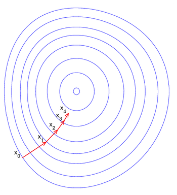
The preconditioner is applied to the gradient:

Preconditioning here can be viewed as changing the geometry of the vector space with the goal to make the level sets look like circles. In this case the preconditioned gradient aims closer to the point of the extrema as on the figure, which speeds up the convergence.
 ,
,
where and
and  are real column-vectors and
  is a real symmetric positive-definite matrix
, is exactly the solution of the linear equation . Since
  , the preconditioned gradient descent
method of minimizing is
is

This is the preconditioned Richardson iteration for solving a system of linear equations.

where is a real non-zero column-vector and
  is a real symmetric positive-definite matrix
, is the smallest eigenvalue of , while the minimizer is the corresponding eigenvector. Since
  is proportional to
  , the preconditioned gradient descent
method of minimizing is
is

This is an analog of preconditioned Richardson iteration for solving eigenvalue problems.

One should have in mind, however, that constructing an efficient preconditioner is very often computationally expensive. The increased cost of updating the preconditioner can easily override the positive effect of faster convergence.
Mathematics
Mathematics is the study of quantity, space, structure, and change. Mathematicians seek out patterns and formulate new conjectures. Mathematicians resolve the truth or falsity of conjectures by mathematical proofs, which are arguments sufficient to convince other mathematicians of their validity...
, preconditioning is a procedure of an application of a transformation, called the preconditioner, that conditions a given problem into a form that is more suitable for numerical solution. Preconditioning is typically related to reducing a condition number
Condition number
In the field of numerical analysis, the condition number of a function with respect to an argument measures the asymptotically worst case of how much the function can change in proportion to small changes in the argument...
of the problem. The preconditioned problem is then usually solved by an iterative method
Iterative method
In computational mathematics, an iterative method is a mathematical procedure that generates a sequence of improving approximate solutions for a class of problems. A specific implementation of an iterative method, including the termination criteria, is an algorithm of the iterative method...
.
Preconditioning for linear systems
In linear algebraLinear algebra
Linear algebra is a branch of mathematics that studies vector spaces, also called linear spaces, along with linear functions that input one vector and output another. Such functions are called linear maps and can be represented by matrices if a basis is given. Thus matrix theory is often...
and numerical analysis
Numerical analysis
Numerical analysis is the study of algorithms that use numerical approximation for the problems of mathematical analysis ....
, a preconditioner
of a matrix is a matrix such that has a smaller condition numberCondition number
In the field of numerical analysis, the condition number of a function with respect to an argument measures the asymptotically worst case of how much the function can change in proportion to small changes in the argument...
than
. It is also common to call the preconditioner, rather than , since itself is rarely explicitly available. In modern preconditioning, the application of , i.e., multiplication of a column vector, or a block of column vectors, by , is commonly performed by rather sophisticated computer software packages in a matrix-free fashionMatrix-free methods
In computational mathematics, a matrix-free method is an algorithm for solving a linear system of equations or an eigenvalue problem that does not store the coefficient matrix explicitly, but accesses the matrix by evaluating matrix-vector products...
, i.e., where neither
, nor (and often not even ) are explicitly available in a matrix form.Preconditioners are useful in iterative methods to solve a linear system
for since the rate of convergenceRate of convergence
In numerical analysis, the speed at which a convergent sequence approaches its limit is called the rate of convergence. Although strictly speaking, a limit does not give information about any finite first part of the sequence, this concept is of practical importance if we deal with a sequence of...
for most iterative linear solvers increases as the condition number
Condition number
In the field of numerical analysis, the condition number of a function with respect to an argument measures the asymptotically worst case of how much the function can change in proportion to small changes in the argument...
of a matrix decreases as a result of preconditioning. Preconditioned iterative solvers typically outperform direct solvers, e.g., Gaussian elimination
Gaussian elimination
In linear algebra, Gaussian elimination is an algorithm for solving systems of linear equations. It can also be used to find the rank of a matrix, to calculate the determinant of a matrix, and to calculate the inverse of an invertible square matrix...
, for large, especially for sparse
Sparse matrix
In the subfield of numerical analysis, a sparse matrix is a matrix populated primarily with zeros . The term itself was coined by Harry M. Markowitz....
, matrices. Iterative solvers can be used as matrix-free methods
Matrix-free methods
In computational mathematics, a matrix-free method is an algorithm for solving a linear system of equations or an eigenvalue problem that does not store the coefficient matrix explicitly, but accesses the matrix by evaluating matrix-vector products...
, i.e. become the only choice if the coefficient matrix
is not stored explicitly, but is accessed by evaluating matrix-vector products.Description
Instead of solving the original linear system above, one may solve either the right preconditioned system:
via solving

for
and
for
; or the left preconditioned system:
both of which give the same solution as the original system so long as the preconditioner matrix P is nonsingular. The left preconditioning is more common.
The goal of this preconditioned system is to reduce the condition number
Condition number
In the field of numerical analysis, the condition number of a function with respect to an argument measures the asymptotically worst case of how much the function can change in proportion to small changes in the argument...
of the left or right preconditioned system matrix
or respectively. The preconditioned matrix or is almost never explicitly formed. Only the action of applying the preconditioner solve operation to a given vector need be computed in iterative methods.Typically there is a trade-off in the choice of
. Since the operator must be applied at each step of the iterative linear solver, it should have a small cost (computing time) of applying the operation. The cheapest preconditioner would therefore be since then Clearly, this results in the original linear system and the preconditioner does nothing. At the other extreme, the choice gives which has optimal condition numberCondition number
In the field of numerical analysis, the condition number of a function with respect to an argument measures the asymptotically worst case of how much the function can change in proportion to small changes in the argument...
of 1, requiring a single iteration for convergence; however in this case
and the preconditioner solve is as difficult as solving the original system. One therefore chooses as somewhere between these two extremes, in an attempt to achieve a minimal number of linear iterations while keeping the operator as simple as possible. Some examples of typical preconditioning approaches are detailed below.Preconditioned iterative methods
Preconditioned iterative methods for are, in most cases, mathematically equivalent to standard iterative methods applied to the preconditioned system For example, the standard Richardson iteration for solving isApplied to the preconditioned system
it turns into a preconditioned methodExamples of popular preconditioned iterative methods for linear systems include the preconditioned conjugate gradient method, the biconjugate gradient method
Biconjugate gradient method
In mathematics, more specifically in numerical linear algebra, the biconjugate gradient method is an algorithm to solve systems of linear equationsA x= b.\,...
, and generalized minimal residual method
Generalized minimal residual method
In mathematics, the generalized minimal residual method is an iterative method for the numerical solution of a system of linear equations. The method approximates the solution by the vector in a Krylov subspace with minimal residual. The Arnoldi iteration is used to find this vector.The GMRES...
. Iterative methods, which use scalar products to compute the iterative parameters, require corresponding changes in the scalar product together with substituting
for Geometric interpretation
For a symmetric positive definitePositive-definite matrix
In linear algebra, a positive-definite matrix is a matrix that in many ways is analogous to a positive real number. The notion is closely related to a positive-definite symmetric bilinear form ....
matrix
the preconditioner is typically chosen to be symmetric positive definite as well. The preconditioned operator is then also symmetric positive definite, but with respect to the -based scalar product. In this case, the desired effect in applying a preconditioner is to make the quadratic formQuadratic form
In mathematics, a quadratic form is a homogeneous polynomial of degree two in a number of variables. For example,4x^2 + 2xy - 3y^2\,\!is a quadratic form in the variables x and y....
of the preconditioned operator
with respect to the -based scalar product to be nearly sphericalhttp://www.cs.cmu.edu/~quake-papers/painless-conjugate-gradient.pdf.Variable and non-linear preconditioning
Denoting, we highlight that preconditioning is practically implemented as multiplying some vector by , i.e., computing the product . In many applications, is not given as a matrix, but rather as an operator acting on the vector . Some popular preconditioners, however, change with and the dependence on may not be linear. Typical examples involve using non-linear iterative methods, e.g., the conjugate gradient methodConjugate gradient method
In mathematics, the conjugate gradient method is an algorithm for the numerical solution of particular systems of linear equations, namely those whose matrix is symmetric and positive-definite. The conjugate gradient method is an iterative method, so it can be applied to sparse systems that are too...
, as a part of the preconditioner construction. Such preconditioners may be practically very efficient, however, their behavior is hard to predict theoretically.
Spectrally equivalent preconditioning
The most common use of preconditioning is for iterative solution of linear systems resulting from approximations of partial differential equations. The better the approximation quality, the larger the matrix size is. In such a case, the goal of optimal preconditioning is, on the one side, to make the spectral condition number of to be bounded from above by a constant independent in the matrix size, which is called spectrally equivalent preconditioning by D'yakonovEvgenii Georgievich D'yakonov
Evgenii Georgievich D'yakonov was a Russian mathematician.D'yakonov was a Ph.D. student of Sergei Sobolev. He worked at the Moscow State University. He authored over hundred papers and several books...
. On the other hand, the cost of application of the
should ideally be proportional (also independent in the matrix size) to the cost of multiplication of by a vector.Jacobi (or diagonal) preconditioner
The Jacobi preconditioner is one of the simplest forms of preconditioning, in which the preconditioner is chosen to be the diagonal of the matrix Assuming , we get It is efficient for diagonally dominant matricesDiagonally dominant matrix
In mathematics, a matrix is said to be diagonally dominant if for every row of the matrix, the magnitude of the diagonal entry in a row is larger than or equal to the sum of the magnitudes of all the other entries in that row...
.SPAI
The Sparse Approximate Inverse preconditioner minimises where is the Frobenius matrix norm and is from some suitably constrained set of sparse matrices. Under the Frobenius norm, this reduces to solving numerous independent least-squares problems (one for every column). The entries in must be restricted to some sparsity pattern or the problem becomes as hard and time consuming as finding the exact inverse of . This method, as well as means to select sparsity patterns, were introduced by [M.J. Grote, T. Huckle, SIAM J. Sci. Comput . 18 (1997) 838–853].Other preconditioners
- Incomplete Cholesky factorizationIncomplete Cholesky factorizationIn numerical analysis, an incomplete Cholesky factorization of a symmetric positive definite matrix is a sparse approximation of the Cholesky factorization...
- Incomplete LU factorizationIncomplete LU factorizationIn numerical analysis, a field within mathematics, an incomplete LU factorization of a matrix is an sparse approximation of the LU factorization. Incomplete LU factorization is often used as a preconditioner.-External links:*...
- Successive over-relaxationSuccessive over-relaxationIn numerical linear algebra, the method of successive over-relaxation is a variant of the Gauss–Seidel method for solving a linear system of equations, resulting in faster convergence. A similar method can be used for any slowly converging iterative process.It was devised simultaneously by David...
- Multigrid#Multigrid preconditioning
External links
- Preconditioned Conjugate Gradient – math-linux.com
- Templates for the Solution of Linear Systems: Building Blocks for Iterative Methods
Preconditioning for eigenvalue problems
Eigenvalue problems can be framed in several alternative ways, each leading to its own preconditioning. The traditional preconditioning is based on the so-called spectral transformations. Knowing (approximately) the targeted eigenvalue, one can compute the corresponding eigenvector by solving the related homogeneous linear system, thus allowing to use preconditioning for linear system. Finally, formulating the eigenvalue problem as optimization of the Rayleigh quotient brings preconditioned optimization techniques to the scene.Spectral transformations
By analogy with linear systems, for an eigenvalue problem one may be tempted to replace the matrix with the matrix using a preconditioner . However, this makes sense only if the seeking eigenvectors of and are the same. This is the case for spectral transformations.The most popular spectral transformation is the so-called shift-and-invert transformation, where for a given scalar
, called the shift, the original eigenvalue problem is replaced with the shift-and-invert problem . The eigenvectors are preserved, and one can solve the shift-and-invert problem by an iterative solver, e.g., the power iterationPower iteration
In mathematics, the power iteration is an eigenvalue algorithm: given a matrix A, the algorithm will produce a number λ and a nonzero vector v , such that Av = λv....
. This gives the Inverse iteration
Inverse iteration
In numerical analysis, inverse iteration is an iterative eigenvalue algorithm. It allows to find an approximateeigenvector when an approximation to a corresponding eigenvalue is already known....
, which normally converges to the eigenvector, corresponding to the eigenvalue closest to the shift
. The Rayleigh quotient iterationRayleigh quotient iteration
Rayleigh quotient iteration is an eigenvalue algorithm which extends the idea of the inverse iteration by using the Rayleigh quotient to obtain increasingly accurate eigenvalue estimates....
is a shift-and-invert method with a variable shift.
Spectral transformations are specific for eigenvalue problems and have no analogs for linear systems. They require accurate numerical calculation of the transformation involved, which becomes the main bottleneck for large problems.
General preconditioning
To make a close connection to linear systems, let us suppose that the targeted eigenvalue is known (approximately). Then one can compute the corresponding eigenvector from the homogeneous linear system . Using the concept of left preconditioning for linear systems, we obtain , where is the preconditioner, which we can try to solve using the Richardson iterationThe ideal preconditioning
The Moore–Penrose pseudoinverse is the preconditioner, which makes the Richardson iteration above converge in one step with , since , denoted by , is the orthogonal projector on the eigenspace, corresponding to . The choice is impractical for three independent reasons. First, is actually not known, although it can be replaced with its approximation . Second, the exact Moore–Penrose pseudoinverse requires the knowledge of the eigenvector, which we are trying to find. This can be somewhat circumvented by the use of the Jacobi-Davidson preconditioner , where approximates . Last, but not least, this approach requires accurate numerical solution of linear system with the system matrix , which becomes as expensive for large problems as the shift-and-invert method above. If the solution is not accurate enough, step two may be redundant.Practical preconditioning
Let us first replace the theoretical value in the Richardson iteration above with its current approximation to obtain a practical algorithmA popular choice is
using the Rayleigh quotient function . Practical preconditioning may be as trivial as just using or For some classes of eigenvalue problems the efficiency of has been demonstrated, both numerically and theoretically. The choice allows one to easily utilize for eigenvalue problems the vast variety of preconditioners developed for linear systems.Due to the changing value
, a comprehensive theoretical convergence analysis is much more difficult, compared to the linear systems case, even for the simplest methods, such as the Richardson iteration.External links
Preconditioning in optimization
Optimization (mathematics)
In mathematics, computational science, or management science, mathematical optimization refers to the selection of a best element from some set of available alternatives....
, preconditioning is typically used to accelerate first-order optimization
Optimization (mathematics)
In mathematics, computational science, or management science, mathematical optimization refers to the selection of a best element from some set of available alternatives....
algorithms.
Description
For example, to find a local minimum of a real-valued function using gradient descentGradient descent
Gradient descent is a first-order optimization algorithm. To find a local minimum of a function using gradient descent, one takes steps proportional to the negative of the gradient of the function at the current point...
, one takes steps proportional to the negative of the gradient
Gradient
In vector calculus, the gradient of a scalar field is a vector field that points in the direction of the greatest rate of increase of the scalar field, and whose magnitude is the greatest rate of change....
(or of the approximate gradient) of the function at the current point:The preconditioner is applied to the gradient:
Preconditioning here can be viewed as changing the geometry of the vector space with the goal to make the level sets look like circles. In this case the preconditioned gradient aims closer to the point of the extrema as on the figure, which speeds up the convergence.
Connection to linear systems
The minimum of a quadratic function,where
and are real column-vectors and is a real symmetric positive-definite matrixPositive-definite matrix
In linear algebra, a positive-definite matrix is a matrix that in many ways is analogous to a positive real number. The notion is closely related to a positive-definite symmetric bilinear form ....
, is exactly the solution of the linear equation
. Since , the preconditioned gradient descentGradient descent
Gradient descent is a first-order optimization algorithm. To find a local minimum of a function using gradient descent, one takes steps proportional to the negative of the gradient of the function at the current point...
method of minimizing
isThis is the preconditioned Richardson iteration for solving a system of linear equations.
Connection to eigenvalue problems
The minimum of the Rayleigh quotientwhere
is a real non-zero column-vector and is a real symmetric positive-definite matrixPositive-definite matrix
In linear algebra, a positive-definite matrix is a matrix that in many ways is analogous to a positive real number. The notion is closely related to a positive-definite symmetric bilinear form ....
, is the smallest eigenvalue of
, while the minimizer is the corresponding eigenvector. Since is proportional to , the preconditioned gradient descentGradient descent
Gradient descent is a first-order optimization algorithm. To find a local minimum of a function using gradient descent, one takes steps proportional to the negative of the gradient of the function at the current point...
method of minimizing
isThis is an analog of preconditioned Richardson iteration for solving eigenvalue problems.
Variable preconditioning
In many cases, it may be beneficial to change the preconditioner at some or even every step of an iterative algorithm in order to accommodate for a changing shape of the level sets, as inOne should have in mind, however, that constructing an efficient preconditioner is very often computationally expensive. The increased cost of updating the preconditioner can easily override the positive effect of faster convergence.