
Hilbert transform
Encyclopedia
In mathematics
and in signal processing
, the Hilbert transform is a linear operator which takes a function, u(t), and produces a function, H(u(t)), with the same domain
. The Hilbert transform is named after David Hilbert
, who first introduced the operator in order to solve a special case of the Riemann–Hilbert problem for holomorphic function
s. It is a basic tool in Fourier analysis, and provides a concrete means for realizing the harmonic conjugate
of a given function or Fourier series
. Furthermore, in harmonic analysis
, it is an example of a singular integral operator
, and of a Fourier multiplier
. The Hilbert transform is also important in the field of signal processing where it is used to derive the analytic representation
of a signal u(t).
The Hilbert transform was originally defined for periodic function
s, or equivalently for functions on the circle
, in which case it is given by convolution
with the Hilbert kernel. More commonly, however, the Hilbert transform refers to a convolution with the Cauchy kernel, for functions defined on the real line
R (the boundary
of the upper half-plane). The Hilbert transform is closely related to the Paley–Wiener theorem
, another result relating holomorphic functions in the upper half-plane and Fourier transform
s of functions on the real line.

of u(t) with the function h(t) = 1/(π t). Because h(t) is not integrable the integrals defining the convolution do not converge. Instead, the Hilbert transform is defined using the Cauchy principal value
(denoted here by p.v.) Explicitly, the Hilbert transform of a function (or signal) u(t) is given by
provided this integral exists as a principal value. This is precisely the convolution of u with the tempered distribution
p.v. 1/πt . Alternatively, by changing variables, the principal value integral can be written explicitly as

When the Hilbert transform is applied twice in succession to a function u, the result is minus u:

provided the integrals defining both iterations converge in a suitable sense. In particular, the inverse transform is −H. This fact can most easily be seen by considering the effect of the Hilbert transform on the Fourier transform of (see Relationship with the Fourier transform, below).
For an analytic function
in upper half-plane the Hilbert transform describes the relationship between the real part and the imaginary part of the boundary values. That is, if f(z) is analytic in the plane Im z > 0 and u(t) = Re f(t + 0·i ) then Im f(t + 0·i ) = H(u)(t) up to an additive constant, provided this Hilbert transform exists.
the Hilbert transform of u(t) is commonly denoted by However, in mathematics, this notation is already extensively used to denote the Fourier transform of u(t). Occasionally, the Hilbert transform may be denoted by
  . Furthermore, many sources define the Hilbert transform as the negative of the one defined here.
. In 1928, Marcel Riesz
proved that the Hilbert transform can be defined for u in Lp(R)
for 1 < p < ∞, that the Hilbert transform is a bounded operator
on Lp(R) for the same range of p, and that similar results hold for the Hilbert transform on the circle as well as the discrete Hilbert transform . The Hilbert transform was a motivating example for Antoni Zygmund
and Alberto Calderón
during their study of singular integral
s . Their investigations have played a fundamental role in modern harmonic analysis. Various generalizations of the Hilbert transform, such as the bilinear and trilinear Hilbert transforms are still active areas of research today.
The early 2000s saw the development of Hilbert spectroscopy
which uses Hilbert transforms to detect signatures of chemical mixtures by analyzing broad spectrum signals from gigahertz to terahertz frequency radio.
. The symbol of H is σH(ω) = −i sgn(ω) where sgn is the signum function
. Therefore:

where denotes the Fourier transform
. Since sgn(x) = sgn(2πx), it follows that this result applies to the three common definitions of
By Euler's formula
,
Therefore H(u)(t) has the effect of shifting the phase of the negative frequency
components of u(t) by +90° (π/2 radians) and the phase of the positive frequency components by −90°. And i·H(u)(t) has the effect of restoring the positive frequency components while shifting the negative frequency ones an additional +90°, resulting in their negation.
When the Hilbert transform is applied twice, the phase of the negative and positive frequency components of u(t) are respectively shifted by +180° and −180°, which are equivalent amounts. The signal is negated, i.e., H(H(u)) = −u, because:

Notes
An extensive table of Hilbert transforms is available .
Note that the Hilbert transform of a constant is zero.
for 1
More precisely, if u is in Lp(R) for 1
exists for almost every t. The limit function is also in Lp(R), and is in fact the limit in the mean of the improper integral as well. That is,

as ε→0 in the Lp-norm, as well as pointwise almost everywhere, by the Titchmarsh theorem
.
In the case p=1, the Hilbert transform still converges pointwise almost everywhere, but may fail to be itself integrable even locally . In particular, convergence in the mean does not in general happen in this case. The Hilbert transform of an L1 function does converge, however, in L1-weak, and the Hilbert transform is a bounded operator from L1 to L1,w . (In particular, since the Hilbert transform is also a multiplier operator on L2, Marcinkiewicz interpolation and a duality argument furnishes an alternative proof that H is bounded on Lp.)
p (R) is a bounded linear operator, meaning that there exists a constant Cp such that

for all u∈Lp(R). This theorem is due to ; see also .
The best constant Cp is given by
This result is due to ; see also . The same best constants hold for the periodic Hilbert transform.
The boundedness of the Hilbert transform implies the Lp(R) convergence of the (symmetric) Fourier series of periodic functions in Lp(R), see for example

for u ∈ Lp(R) and v ∈ Lq(R) .

provided each transform is well-defined. Since H preserves the space Lp(R), this implies in particular that the Hilbert transform is invertible on Lp(R), and that


Iterating this identity,

This is rigorously true as stated provided u and its first k derivatives belong to Lp(R) .
with the tempered distribution

Thus formally,

However, a priori this may only be defined for u a distribution of compact support. It is possible to work somewhat rigorously with this since compactly supported functions (which are distributions a fortiori) are dense in Lp. Alternatively, one may use the fact that h(t) is the distributional derivative of the function log|t|/π; to wit

For most operational purposes the Hilbert transform can be treated as a convolution. For example, in a formal sense, the Hilbert transform of a convolution is the convolution of the Hilbert transform on either factor:

This is rigorously true if u and v are compactly supported distributions since, in that case,

By passing to an appropriate limit, it is thus also true if u ∈ Lp and v ∈ Lr provided

a theorem due to .
Up to a multiplicative constant, the Hilbert transform is the only L2 bounded operator with these properties .
. Since the Hilbert transform commutes with differentiation, and is a bounded operator on Lp, H restricts to give a continuous transform on the inverse limit
of Sobolev spaces:

The Hilbert transform can then be defined on the dual space of , denoted
  , consisting of Lp distributions. This is accomplished by the duality pairing: for
  , define
  by
by

for all .
.
It is possible to define the Hilbert transform on the space of tempered distributions as well by an approach due to , but considerably more care is needed because of the singularity in the integral.
of bounded mean oscillation
(BMO) classes.
Interpreted naively, the Hilbert transform of a bounded function is clearly ill-defined. For instance, with u = sgn(x), the integral defining H(u) diverges almost everywhere to ±∞. To alleviate such difficulties, the Hilbert transform of an L∞-function is therefore defined by the following regularized
form of the integral

where as above h(x) = 1/πx and

The modified transform H agrees with the original transform on functions of compact support by a general result of ; see . The resulting integral, furthermore, converges pointwise almost everywhere, and with respect to the BMO norm, to a function of bounded mean oscillation.
A deep result of and is that a function is of bounded mean oscillation if and only if it has the form ƒ + H(g) for some ƒ, g ∈ L∞(R).

is the boundary value of a holomorphic function
F(z) in the upper half-plane. Under these circumstances, if f and g are sufficiently integrable, then one is the Hilbert transform of the other.
Suppose that f ∈ Lp(R). Then, by the theory of the Poisson integral, f admits a unique harmonic extension into the upper half-plane, and this extension is given by

which is the convolution of f with the Poisson kernel

Furthermore, there is a unique harmonic function v defined in the upper half-plane such that F(z) = u(z) + iv(z) is holomorphic and
This harmonic function is obtained from f by taking a convolution with the conjugate Poisson kernel

Thus
Indeed, the real and imaginary parts of the Cauchy kernel are
so that F = u + iv is holomorphic by Cauchy's theorem.
The function v obtained from u in this way is called the harmonic conjugate
of u. The (non-tangential) boundary limit of v(x,y) as y → 0 is the Hilbert transform of f. Thus, succinctly,
makes precise the relationship between the boundary values of holomorphic functions in the upper half-plane and the Hilbert transform . It gives necessary and sufficient conditions for a complex-valued square-integrable function F(x) on the real line to be the boundary value of a function in the Hardy space
H2(U) of holomorphic functions in the upper half-plane U.
The theorem states that the following conditions for a complex-valued square-integrable function F : R → C are equivalent:
A weaker result is true for functions of class Lp
for p > 1 . Specifically, if F(z) is a holomorphic function such that

for all y, then there is a complex-valued function F(x) in Lp(R) such that F(x + iy) → F(x) in the Lp norm as y → 0 (as well as holding pointwise almost everywhere
). Furthermore,

where ƒ is a real-valued function in Lp(R) and g is the Hilbert transform (of class Lp) of ƒ.
This is not true in the case p = 1. In fact, the Hilbert transform of an L1 function ƒ need not converge in the mean to another L1 function. Nevertheless , the Hilbert transform of ƒ does converge almost everywhere to a finite function g such that

This result is directly analogous to one by Andrey Kolmogorov
for Hardy functions in the disc .
on the upper half-plane and F− is holomorphic on the lower half-plane, such that for x along the real axis,
where f(x) is some given real-valued function of x ∈ R. The left-hand side of this equation may be understood either as the difference of the limits of F± from the appropriate half-planes, or as a hyperfunction
distribution. Two functions of this form are a solution of the Riemann–Hilbert problem.
Formally, if F± solve the Riemann–Hilbert problem
then the Hilbert transform of f(x) is given by

The circular Hilbert transform is used in giving a characterization of Hardy space and in the study of the conjugate function in Fourier series. The kernel is known as the Hilbert kernel since it was in this form the Hilbert transform was originally studied .
The Hilbert kernel (for the circular Hilbert transform) can be obtained by making the Cauchy kernel 1/x periodic. More precisely, for x≠0

Many results about the circular Hilbert transform may be derived from the corresponding results for the Hilbert transform from this correspondence.

where and
and  are the low- and high-pass signals respectively.
Amplitude modulated signals are modeled as the product of a bandlimited
"message" waveform, um(t), and a sinusoidal "carrier":

When has no frequency content above the carrier frequency,
  then by Bedrosian's theorem:

So, the Hilbert transform may be seen as simple as a circuit that produces a 90° phase shift at the carrier frequency. Furthermore:
from which one can reconstruct the carrier waveform. Then the message can be extracted from u(t) by coherent demodulation.

For the narrowband model [above], the analytic representation is:
This complex heterodyne
operation shifts all the frequency components of um(t) above 0 Hz. In that case, the imaginary part of the result is a Hilbert transform of the real part. This is an indirect way to produce Hilbert transforms.
While the analytic representation of a signal is not necessarily an analytic function
, ua(t) is given by the boundary values of an analytic function in the upper half-plane.

is called phase (or frequency) modulation
. The instantaneous frequency is For sufficiently large
  compared to
  :
:

and:

 in is also an analytic representation (of a message waveform), that is:

the result is single-sideband modulation:

whose transmitted component is:

and therefore cannot be implemented as is, if u is a time-dependent signal. If u is a function of a non-temporal variable, e.g., spatial, the non-causality might not be a problem. The filter is also of infinite support
which may be a problem in certain applications. Another issue relates to what happens with the zero frequency (DC), which can be avoided by assuring that does not contain a DC-component.
A practical implementation in many cases implies that a finite support filter, which in addition is made causal by means of a suitable delay, is used to approximate the computation. The approximation may also imply that only a specific frequency range is subject to the characteristic phase shift related to the Hilbert transform. See also quadrature filter.

which is the discrete-time Fourier transform
of the infinite sequence:

If a signal is bandlimited
, then is bandlimited in the same way. Consequently, both these signals can be sampled according to the sampling theorem, resulting in the discrete signals
  and
and  The relation between the two discrete signals is then given by the convolution:

When an FIR
approximation is substituted for we see rolloff of the passband at the low and high ends (0 and Nyquist), resulting in a bandpass filter as shown in the figure above. The high end can be restored by an FIR that more closely resembles samples of the smooth, continuous-time
  as shown in the next figure. But as a practical matter, a properly-sampled
  sequence has no useful components at those frequencies.
As the impulse response gets longer, the low end frequencies are also restored. Hilbert studied the transform :
and showed that for in ℓ2 the sequence
  is also in ℓ2. An elementary proof of this fact can be found in . This discrete Hilbert transform was used by E. C. Titchmarsh to give alternate proofs of the results of M. Riesz in the continuous case .
 We also note that a sequence similar to
  can be generated by sampling σH(ω) and computing the inverse discrete Fourier transform
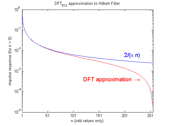
. The larger the transform (i.e., more samples per radians), the better the agreement (for a given value of the abscissa, n). The figure shows the comparison for a 512-point transform. (Due to odd-symmetry, only half the sequence is actually plotted.)
But that is not the actual point, because it is easier and more accurate to generate directly from the formula. The point is that many applications choose to avoid the convolution by doing the equivalent frequency-domain operation: simple multiplication of the signal transform with σH(ω), made even easier by the fact that the real and imaginary components are 0 and ±1 respectively. The attractiveness of that approach is only apparent when the actual Fourier transforms are replaced by samples of the same, i.e., the DFT, which is an approximation and introduces some distortion. Thus, after transforming back to the time-domain, those applications have indirectly generated (and convolved with) not
  , but the DFT approximation to it, which is shown in the figure.
Notes on fast convolution:
Mathematics
Mathematics is the study of quantity, space, structure, and change. Mathematicians seek out patterns and formulate new conjectures. Mathematicians resolve the truth or falsity of conjectures by mathematical proofs, which are arguments sufficient to convince other mathematicians of their validity...
and in signal processing
Signal processing
Signal processing is an area of systems engineering, electrical engineering and applied mathematics that deals with operations on or analysis of signals, in either discrete or continuous time...
, the Hilbert transform is a linear operator which takes a function, u(t), and produces a function, H(u(t)), with the same domain
Domain (mathematics)
In mathematics, the domain of definition or simply the domain of a function is the set of "input" or argument values for which the function is defined...
. The Hilbert transform is named after David Hilbert
David Hilbert
David Hilbert was a German mathematician. He is recognized as one of the most influential and universal mathematicians of the 19th and early 20th centuries. Hilbert discovered and developed a broad range of fundamental ideas in many areas, including invariant theory and the axiomatization of...
, who first introduced the operator in order to solve a special case of the Riemann–Hilbert problem for holomorphic function
Holomorphic function
In mathematics, holomorphic functions are the central objects of study in complex analysis. A holomorphic function is a complex-valued function of one or more complex variables that is complex differentiable in a neighborhood of every point in its domain...
s. It is a basic tool in Fourier analysis, and provides a concrete means for realizing the harmonic conjugate
Harmonic conjugate
In mathematics, a function u defined on some open domain \Omega\subset\R^2 is said to have as a conjugate a function v if and only if they are respectively real and imaginary part of a holomorphic function f of the complex variable z:=x+iy\in\Omega. That is, v is conjugated to u if f:=u+iv is...
of a given function or Fourier series
Fourier series
In mathematics, a Fourier series decomposes periodic functions or periodic signals into the sum of a set of simple oscillating functions, namely sines and cosines...
. Furthermore, in harmonic analysis
Harmonic analysis
Harmonic analysis is the branch of mathematics that studies the representation of functions or signals as the superposition of basic waves. It investigates and generalizes the notions of Fourier series and Fourier transforms...
, it is an example of a singular integral operator
Singular integral
In mathematics, singular integrals are central to harmonic analysis and are intimately connected with the study of partial differential equations. Broadly speaking a singular integral is an integral operator...
, and of a Fourier multiplier
Multiplier (Fourier analysis)
In Fourier analysis, a multiplier operator is a type of linear operator, or transformation of functions. These operators act on a function by altering its Fourier transform. Specifically they multiply the Fourier transform of a function by a specified function known as the multiplier or symbol...
. The Hilbert transform is also important in the field of signal processing where it is used to derive the analytic representation
Analytic signal
In mathematics and signal processing, the analytic representation of a real-valued function or signal facilitates many mathematical manipulations of the signal. The basic idea is that the negative frequency components of the Fourier transform of a real-valued function are superfluous, due to the...
of a signal u(t).
The Hilbert transform was originally defined for periodic function
Periodic function
In mathematics, a periodic function is a function that repeats its values in regular intervals or periods. The most important examples are the trigonometric functions, which repeat over intervals of length 2π radians. Periodic functions are used throughout science to describe oscillations,...
s, or equivalently for functions on the circle
Circle
A circle is a simple shape of Euclidean geometry consisting of those points in a plane that are a given distance from a given point, the centre. The distance between any of the points and the centre is called the radius....
, in which case it is given by convolution
Convolution
In mathematics and, in particular, functional analysis, convolution is a mathematical operation on two functions f and g, producing a third function that is typically viewed as a modified version of one of the original functions. Convolution is similar to cross-correlation...
with the Hilbert kernel. More commonly, however, the Hilbert transform refers to a convolution with the Cauchy kernel, for functions defined on the real line
Real line
In mathematics, the real line, or real number line is the line whose points are the real numbers. That is, the real line is the set of all real numbers, viewed as a geometric space, namely the Euclidean space of dimension one...
R (the boundary
Boundary (topology)
In topology and mathematics in general, the boundary of a subset S of a topological space X is the set of points which can be approached both from S and from the outside of S. More precisely, it is the set of points in the closure of S, not belonging to the interior of S. An element of the boundary...
of the upper half-plane). The Hilbert transform is closely related to the Paley–Wiener theorem
Paley–Wiener theorem
In mathematics, a Paley–Wiener theorem is any theorem that relates decay properties of a function or distribution at infinity with analyticity of its Fourier transform. The theorem is named for Raymond Paley and Norbert Wiener . The original theorems did not use the language of distributions,...
, another result relating holomorphic functions in the upper half-plane and Fourier transform
Fourier transform
In mathematics, Fourier analysis is a subject area which grew from the study of Fourier series. The subject began with the study of the way general functions may be represented by sums of simpler trigonometric functions...
s of functions on the real line.
Introduction
The Hilbert transform can be thought of as the convolutionConvolution
In mathematics and, in particular, functional analysis, convolution is a mathematical operation on two functions f and g, producing a third function that is typically viewed as a modified version of one of the original functions. Convolution is similar to cross-correlation...
of u(t) with the function h(t) = 1/(π t). Because h(t) is not integrable the integrals defining the convolution do not converge. Instead, the Hilbert transform is defined using the Cauchy principal value
Cauchy principal value
In mathematics, the Cauchy principal value, named after Augustin Louis Cauchy, is a method for assigning values to certain improper integrals which would otherwise be undefined.-Formulation:...
(denoted here by p.v.) Explicitly, the Hilbert transform of a function (or signal) u(t) is given by
provided this integral exists as a principal value. This is precisely the convolution of u with the tempered distribution
Tempered distribution
*Distribution *Tempered representation...
p.v. 1/πt . Alternatively, by changing variables, the principal value integral can be written explicitly as
When the Hilbert transform is applied twice in succession to a function u, the result is minus u:
provided the integrals defining both iterations converge in a suitable sense. In particular, the inverse transform is −H. This fact can most easily be seen by considering the effect of the Hilbert transform on the Fourier transform of
(see Relationship with the Fourier transform, below).For an analytic function
Analytic function
In mathematics, an analytic function is a function that is locally given by a convergent power series. There exist both real analytic functions and complex analytic functions, categories that are similar in some ways, but different in others...
in upper half-plane the Hilbert transform describes the relationship between the real part and the imaginary part of the boundary values. That is, if f(z) is analytic in the plane Im z > 0 and u(t) = Re f(t + 0·i ) then Im f(t + 0·i ) = H(u)(t) up to an additive constant, provided this Hilbert transform exists.
Notation
In signal processingSignal processing
Signal processing is an area of systems engineering, electrical engineering and applied mathematics that deals with operations on or analysis of signals, in either discrete or continuous time...
the Hilbert transform of u(t) is commonly denoted by
However, in mathematics, this notation is already extensively used to denote the Fourier transform of u(t). Occasionally, the Hilbert transform may be denoted by . Furthermore, many sources define the Hilbert transform as the negative of the one defined here.History
The Hilbert transform arose in Hilbert's 1905 work on a problem posed by Riemann concerning analytic functions which has come to be known as the Riemann–Hilbert problem. Hilbert's work was mainly concerned with the Hilbert transform for functions defined on the circle . Some of his earlier work related to the Discrete Hilbert Transform dates back to lectures he gave in Göttingen. The results were later published by Hermann Weyl in his dissertation . Schur improved Hilbert's results about the discrete Hilbert transform and extended them to the integral case . These results were restricted to the spaces L2 and ℓ2Lp space
In mathematics, the Lp spaces are function spaces defined using a natural generalization of the p-norm for finite-dimensional vector spaces...
. In 1928, Marcel Riesz
Marcel Riesz
Marcel Riesz was a Hungarian mathematician who was born in Győr, Hungary . He moved to Sweden in 1908 and spent the rest of his life there, dying in Lund, where he was a professor from 1926 at Lund University...
proved that the Hilbert transform can be defined for u in Lp(R)
Lp space
In mathematics, the Lp spaces are function spaces defined using a natural generalization of the p-norm for finite-dimensional vector spaces...
for 1 < p < ∞, that the Hilbert transform is a bounded operator
Bounded operator
In functional analysis, a branch of mathematics, a bounded linear operator is a linear transformation L between normed vector spaces X and Y for which the ratio of the norm of L to that of v is bounded by the same number, over all non-zero vectors v in X...
on Lp(R) for the same range of p, and that similar results hold for the Hilbert transform on the circle as well as the discrete Hilbert transform . The Hilbert transform was a motivating example for Antoni Zygmund
Antoni Zygmund
Antoni Zygmund was a Polish-born American mathematician.-Life:Born in Warsaw, Zygmund obtained his PhD from Warsaw University and became a professor at Stefan Batory University at Wilno...
and Alberto Calderón
Alberto Calderón
Alberto Pedro Calderón was an Argentine mathematician best known for his work on the theory of partial differential equations and singular integral operators, and widely considered as one of the 20th century's most important mathematicians...
during their study of singular integral
Singular integral
In mathematics, singular integrals are central to harmonic analysis and are intimately connected with the study of partial differential equations. Broadly speaking a singular integral is an integral operator...
s . Their investigations have played a fundamental role in modern harmonic analysis. Various generalizations of the Hilbert transform, such as the bilinear and trilinear Hilbert transforms are still active areas of research today.
The early 2000s saw the development of Hilbert spectroscopy
Hilbert spectroscopy
Hilbert Spectroscopy uses Hilbert transforms to analyze broad spectrum signals from gigahertz to terahertz frequency radio. One suggested use is to quickly analyze liquids inside airport passenger luggage....
which uses Hilbert transforms to detect signatures of chemical mixtures by analyzing broad spectrum signals from gigahertz to terahertz frequency radio.
Relationship with the Fourier transform
As mentioned before, the Hilbert transform is a multiplier operatorMultiplier (Fourier analysis)
In Fourier analysis, a multiplier operator is a type of linear operator, or transformation of functions. These operators act on a function by altering its Fourier transform. Specifically they multiply the Fourier transform of a function by a specified function known as the multiplier or symbol...
. The symbol of H is σH(ω) = −i sgn(ω) where sgn is the signum function
Sign function
In mathematics, the sign function is an odd mathematical function that extracts the sign of a real number. To avoid confusion with the sine function, this function is often called the signum function ....
. Therefore:
where
denotes the Fourier transformFourier transform
In mathematics, Fourier analysis is a subject area which grew from the study of Fourier series. The subject began with the study of the way general functions may be represented by sums of simpler trigonometric functions...
. Since sgn(x) = sgn(2πx), it follows that this result applies to the three common definitions of
By Euler's formula
Euler's formula
Euler's formula, named after Leonhard Euler, is a mathematical formula in complex analysis that establishes the deep relationship between the trigonometric functions and the complex exponential function...
,
Therefore H(u)(t) has the effect of shifting the phase of the negative frequency
Negative frequency
The concept of negative and positive frequency can be as simple as a wheel rotating one way or the other way. A signed value of frequency indicates both the rate and direction of rotation...
components of u(t) by +90° (π/2 radians) and the phase of the positive frequency components by −90°. And i·H(u)(t) has the effect of restoring the positive frequency components while shifting the negative frequency ones an additional +90°, resulting in their negation.
When the Hilbert transform is applied twice, the phase of the negative and positive frequency components of u(t) are respectively shifted by +180° and −180°, which are equivalent amounts. The signal is negated, i.e., H(H(u)) = −u, because:
Table of selected Hilbert transforms
Signal | Hilbert transformSome authors, e.g., Bracewell, use our −H as their definition of the forward transform. A consequence is that the right column of this table would be negated. |
|---|---|
 The Hilbert transform of the sin and cos functions can be defined in a distributional sense, if there is a concern that the integral defining them is otherwise conditionally convergent. In the periodic setting this result holds without any difficulty. The Hilbert transform of the sin and cos functions can be defined in a distributional sense, if there is a concern that the integral defining them is otherwise conditionally convergent. In the periodic setting this result holds without any difficulty. |
 |
 |
 |
 |
 |
Sinc function  |
 |
Rectangular function  |
 |
| Dirac delta function Dirac delta function The Dirac delta function, or δ function, is a generalized function depending on a real parameter such that it is zero for all values of the parameter except when the parameter is zero, and its integral over the parameter from −∞ to ∞ is equal to one. It was introduced by theoretical...  |
 |
Characteristic Function  |
 |
Notes
An extensive table of Hilbert transforms is available .
Note that the Hilbert transform of a constant is zero.
Domain of definition
It is by no means obvious that the Hilbert transform is well-defined at all, as the improper integral defining it must converge in a suitable sense. However, the Hilbert transform is well-defined for a broad class of functions, namely those in Lp(R)Lp space
In mathematics, the Lp spaces are function spaces defined using a natural generalization of the p-norm for finite-dimensional vector spaces...
for 1
More precisely, if u is in Lp(R) for 1
exists for almost every t. The limit function is also in Lp(R), and is in fact the limit in the mean of the improper integral as well. That is,
as ε→0 in the Lp-norm, as well as pointwise almost everywhere, by the Titchmarsh theorem
Titchmarsh theorem
In mathematics, particularly in the area of Fourier analysis, the Titchmarsh theorem may refer to:* The Titchmarsh convolution theorem* The theorem relating real and imaginary parts of the boundary values of a Hp function in the upper half-plane with the Hilbert transform of an Lp function. See...
.
In the case p=1, the Hilbert transform still converges pointwise almost everywhere, but may fail to be itself integrable even locally . In particular, convergence in the mean does not in general happen in this case. The Hilbert transform of an L1 function does converge, however, in L1-weak, and the Hilbert transform is a bounded operator from L1 to L1,w . (In particular, since the Hilbert transform is also a multiplier operator on L2, Marcinkiewicz interpolation and a duality argument furnishes an alternative proof that H is bounded on Lp.)
Boundedness
If 1for all u∈Lp(R). This theorem is due to ; see also .
The best constant Cp is given by
This result is due to ; see also . The same best constants hold for the periodic Hilbert transform.
The boundedness of the Hilbert transform implies the Lp(R) convergence of the (symmetric) Fourier series of periodic functions in Lp(R), see for example
Anti-self adjointness
The Hilbert transform is an anti-self adjoint operator relative to the duality pairing between Lp(R) and the dual space Lq(R), where p and q are Hölder conjugates and 1 < p,q < ∞. Symbolically,for u ∈ Lp(R) and v ∈ Lq(R) .
Inverse transform
The Hilbert transform is an anti-involution, meaning thatprovided each transform is well-defined. Since H preserves the space Lp(R), this implies in particular that the Hilbert transform is invertible on Lp(R), and that
Differentiation
Formally, the derivative of the Hilbert transform is the Hilbert transform of the derivative:Iterating this identity,
This is rigorously true as stated provided u and its first k derivatives belong to Lp(R) .
Convolutions
The Hilbert transform can formally be realized as a convolutionConvolution
In mathematics and, in particular, functional analysis, convolution is a mathematical operation on two functions f and g, producing a third function that is typically viewed as a modified version of one of the original functions. Convolution is similar to cross-correlation...
with the tempered distribution
Tempered distribution
*Distribution *Tempered representation...
Thus formally,
However, a priori this may only be defined for u a distribution of compact support. It is possible to work somewhat rigorously with this since compactly supported functions (which are distributions a fortiori) are dense in Lp. Alternatively, one may use the fact that h(t) is the distributional derivative of the function log|t|/π; to wit
For most operational purposes the Hilbert transform can be treated as a convolution. For example, in a formal sense, the Hilbert transform of a convolution is the convolution of the Hilbert transform on either factor:
This is rigorously true if u and v are compactly supported distributions since, in that case,
By passing to an appropriate limit, it is thus also true if u ∈ Lp and v ∈ Lr provided
a theorem due to .
Invariance
The Hilbert transform has the following invariance properties.- It commutes with translations. That is, it commutes with the operators Taƒ(x) = ƒ(x + a) for all a in Rn
- It commutes with positive dilations. That is it commutes with the operators Mλƒ(x) = ƒ(λx) for all λ > 0.
- It anticommutesAnticommutativityIn mathematics, anticommutativity is the property of an operation that swapping the position of any two arguments negates the result. Anticommutative operations are widely used in algebra, geometry, mathematical analysis and, as a consequence, in physics: they are often called antisymmetric...
with the reflection Rƒ(x) = ƒ(−x).
Up to a multiplicative constant, the Hilbert transform is the only L2 bounded operator with these properties .
Hilbert transform of distributions
It is further possible to extend the Hilbert transform to certain spaces of distributionsDistribution (mathematics)
In mathematical analysis, distributions are objects that generalize functions. Distributions make it possible to differentiate functions whose derivatives do not exist in the classical sense. In particular, any locally integrable function has a distributional derivative...
. Since the Hilbert transform commutes with differentiation, and is a bounded operator on Lp, H restricts to give a continuous transform on the inverse limit
Inverse limit
In mathematics, the inverse limit is a construction which allows one to "glue together" several related objects, the precise manner of the gluing process being specified by morphisms between the objects...
of Sobolev spaces:
The Hilbert transform can then be defined on the dual space of
, denoted , consisting of Lp distributions. This is accomplished by the duality pairing: for , define byfor all
.It is possible to define the Hilbert transform on the space of tempered distributions as well by an approach due to , but considerably more care is needed because of the singularity in the integral.
Hilbert transform of bounded functions
The Hilbert transform can be defined for functions in L∞(R) as well, but it requires some modifications and caveats. Properly understood, the Hilbert transform maps L∞(R) to the Banach spaceBanach space
In mathematics, Banach spaces is the name for complete normed vector spaces, one of the central objects of study in functional analysis. A complete normed vector space is a vector space V with a norm ||·|| such that every Cauchy sequence in V has a limit in V In mathematics, Banach spaces is the...
of bounded mean oscillation
Bounded mean oscillation
In harmonic analysis, a function of bounded mean oscillation, also known as a BMO function, is a real-valued function whose mean oscillation is bounded...
(BMO) classes.
Interpreted naively, the Hilbert transform of a bounded function is clearly ill-defined. For instance, with u = sgn(x), the integral defining H(u) diverges almost everywhere to ±∞. To alleviate such difficulties, the Hilbert transform of an L∞-function is therefore defined by the following regularized
Regularization (physics)
-Introduction:In physics, especially quantum field theory, regularization is a method of dealing with infinite, divergent, and non-sensical expressions by introducing an auxiliary concept of a regulator...
form of the integral
where as above h(x) = 1/πx and
The modified transform H agrees with the original transform on functions of compact support by a general result of ; see . The resulting integral, furthermore, converges pointwise almost everywhere, and with respect to the BMO norm, to a function of bounded mean oscillation.
A deep result of and is that a function is of bounded mean oscillation if and only if it has the form ƒ + H(g) for some ƒ, g ∈ L∞(R).
Conjugate functions
The Hilbert transform can be understood in terms of a pair of functions f(x) and g(x) such that the functionis the boundary value of a holomorphic function
Holomorphic function
In mathematics, holomorphic functions are the central objects of study in complex analysis. A holomorphic function is a complex-valued function of one or more complex variables that is complex differentiable in a neighborhood of every point in its domain...
F(z) in the upper half-plane. Under these circumstances, if f and g are sufficiently integrable, then one is the Hilbert transform of the other.
Suppose that f ∈ Lp(R). Then, by the theory of the Poisson integral, f admits a unique harmonic extension into the upper half-plane, and this extension is given by
which is the convolution of f with the Poisson kernel
Poisson kernel
In potential theory, the Poisson kernel is an integral kernel, used for solving the two-dimensional Laplace equation, given Dirichlet boundary conditions on the unit disc. The kernel can be understood as the derivative of the Green's function for the Laplace equation...
Furthermore, there is a unique harmonic function v defined in the upper half-plane such that F(z) = u(z) + iv(z) is holomorphic and
This harmonic function is obtained from f by taking a convolution with the conjugate Poisson kernel
Thus
Indeed, the real and imaginary parts of the Cauchy kernel are
so that F = u + iv is holomorphic by Cauchy's theorem.
The function v obtained from u in this way is called the harmonic conjugate
Harmonic conjugate
In mathematics, a function u defined on some open domain \Omega\subset\R^2 is said to have as a conjugate a function v if and only if they are respectively real and imaginary part of a holomorphic function f of the complex variable z:=x+iy\in\Omega. That is, v is conjugated to u if f:=u+iv is...
of u. The (non-tangential) boundary limit of v(x,y) as y → 0 is the Hilbert transform of f. Thus, succinctly,
Titchmarsh's theorem
A theorem due to Edward Charles TitchmarshEdward Charles Titchmarsh
Edward Charles "Ted" Titchmarsh was a leading British mathematician.He was educated at King Edward VII School and Balliol College, Oxford, where he began his studies in October 1917....
makes precise the relationship between the boundary values of holomorphic functions in the upper half-plane and the Hilbert transform . It gives necessary and sufficient conditions for a complex-valued square-integrable function F(x) on the real line to be the boundary value of a function in the Hardy space
Hardy space
In complex analysis, the Hardy spaces Hp are certain spaces of holomorphic functions on the unit disk or upper half plane. They were introduced by Frigyes Riesz , who named them after G. H. Hardy, because of the paper...
H2(U) of holomorphic functions in the upper half-plane U.
The theorem states that the following conditions for a complex-valued square-integrable function F : R → C are equivalent:
- F(x) is the limit as z → x of a holomorphic function F(z) in the upper half-plane such that

- −Im(F) is the Hilbert transform of Re(F), where Re(F) and Im(F) are real-valued functions with F = Re(F) + i Im(F).
- The Fourier transformFourier transformIn mathematics, Fourier analysis is a subject area which grew from the study of Fourier series. The subject began with the study of the way general functions may be represented by sums of simpler trigonometric functions...
 vanishes for x < 0.
A weaker result is true for functions of class Lp
Lp space
In mathematics, the Lp spaces are function spaces defined using a natural generalization of the p-norm for finite-dimensional vector spaces...
for p > 1 . Specifically, if F(z) is a holomorphic function such that
for all y, then there is a complex-valued function F(x) in Lp(R) such that F(x + iy) → F(x) in the Lp norm as y → 0 (as well as holding pointwise almost everywhere
Almost everywhere
In measure theory , a property holds almost everywhere if the set of elements for which the property does not hold is a null set, that is, a set of measure zero . In cases where the measure is not complete, it is sufficient that the set is contained within a set of measure zero...
). Furthermore,
where ƒ is a real-valued function in Lp(R) and g is the Hilbert transform (of class Lp) of ƒ.
This is not true in the case p = 1. In fact, the Hilbert transform of an L1 function ƒ need not converge in the mean to another L1 function. Nevertheless , the Hilbert transform of ƒ does converge almost everywhere to a finite function g such that
This result is directly analogous to one by Andrey Kolmogorov
Andrey Kolmogorov
Andrey Nikolaevich Kolmogorov was a Soviet mathematician, preeminent in the 20th century, who advanced various scientific fields, among them probability theory, topology, intuitionistic logic, turbulence, classical mechanics and computational complexity.-Early life:Kolmogorov was born at Tambov...
for Hardy functions in the disc .
Riemann–Hilbert problem
One form of the Riemann–Hilbert problem seeks to identify pairs of functions F+ and F− such that F+ is holomorphicHolomorphic function
In mathematics, holomorphic functions are the central objects of study in complex analysis. A holomorphic function is a complex-valued function of one or more complex variables that is complex differentiable in a neighborhood of every point in its domain...
on the upper half-plane and F− is holomorphic on the lower half-plane, such that for x along the real axis,
where f(x) is some given real-valued function of x ∈ R. The left-hand side of this equation may be understood either as the difference of the limits of F± from the appropriate half-planes, or as a hyperfunction
Hyperfunction
In mathematics, hyperfunctions are generalizations of functions, as a 'jump' from one holomorphic function to another at a boundary, and can be thought of informally as distributions of infinite order...
distribution. Two functions of this form are a solution of the Riemann–Hilbert problem.
Formally, if F± solve the Riemann–Hilbert problem
then the Hilbert transform of f(x) is given by
Hilbert transform on the circle
For a periodic function f the circular Hilbert transform is defined asThe circular Hilbert transform is used in giving a characterization of Hardy space and in the study of the conjugate function in Fourier series. The kernel
is known as the Hilbert kernel since it was in this form the Hilbert transform was originally studied .The Hilbert kernel (for the circular Hilbert transform) can be obtained by making the Cauchy kernel 1/x periodic. More precisely, for x≠0
Many results about the circular Hilbert transform may be derived from the corresponding results for the Hilbert transform from this correspondence.
Narrowband model
Bedrosian's theorem states that the Hilbert transform of the product of a low-pass and a high-pass signal with non-overlapping spectra is given by the product of the low-pass signal and the Hilbert transform of the high-pass signal, orwhere
and are the low- and high-pass signals respectively.Amplitude modulated signals are modeled as the product of a bandlimited
Bandlimited
Bandlimiting is the limiting of a deterministic or stochastic signal's Fourier transform or power spectral density to zero above a certain finite frequency...
"message" waveform, um(t), and a sinusoidal "carrier":
When
has no frequency content above the carrier frequency, then by Bedrosian's theorem: So, the Hilbert transform may be seen as simple as a circuit that produces a 90° phase shift at the carrier frequency. Furthermore:
 |
 |
 (see next section) (see next section) |
from which one can reconstruct the carrier waveform. Then the message can be extracted from u(t) by coherent demodulation.
Analytic representation
The analytic representation of a signal is defined in terms of the Hilbert transform:For the narrowband model [above], the analytic representation is:
 |
 |
 |
This complex heterodyne
Heterodyne
Heterodyning is a radio signal processing technique invented in 1901 by Canadian inventor-engineer Reginald Fessenden where high frequency signals are converted to lower frequencies by combining two frequencies. Heterodyning is useful for frequency shifting information of interest into a useful...
operation shifts all the frequency components of um(t) above 0 Hz. In that case, the imaginary part of the result is a Hilbert transform of the real part. This is an indirect way to produce Hilbert transforms.
While the analytic representation of a signal is not necessarily an analytic function
Analytic function
In mathematics, an analytic function is a function that is locally given by a convergent power series. There exist both real analytic functions and complex analytic functions, categories that are similar in some ways, but different in others...
, ua(t) is given by the boundary values of an analytic function in the upper half-plane.
Phase/Frequency modulation
The form:is called phase (or frequency) modulation
Phase modulation
Phase modulation is a form of modulation that represents information as variations in the instantaneous phase of a carrier wave.Unlike its more popular counterpart, frequency modulation , PM is not very widely used for radio transmissions...
. The instantaneous frequency is
For sufficiently large compared to :and:
Single sideband modulation (SSB)
When in is also an analytic representation (of a message waveform), that is:the result is single-sideband modulation:
whose transmitted component is:
Causality
The function h with h(t) = 1/(π t) is a non-causal filterCausal filter
In signal processing, a causal filter is a linear and time-invariant causal system. The word causal indicates that the filter output depends only on past and present inputs. A filter whose output also depends on future inputs is non-causal. A filter whose output depends only on future inputs is...
and therefore cannot be implemented as is, if u is a time-dependent signal. If u is a function of a non-temporal variable, e.g., spatial, the non-causality might not be a problem. The filter is also of infinite support
Support (mathematics)
In mathematics, the support of a function is the set of points where the function is not zero, or the closure of that set . This concept is used very widely in mathematical analysis...
which may be a problem in certain applications. Another issue relates to what happens with the zero frequency (DC), which can be avoided by assuring that
does not contain a DC-component.A practical implementation in many cases implies that a finite support filter, which in addition is made causal by means of a suitable delay, is used to approximate the computation. The approximation may also imply that only a specific frequency range is subject to the characteristic phase shift related to the Hilbert transform. See also quadrature filter.
Discrete Hilbert transforms
There are two objects of study which are considered discrete Hilbert transforms. The Discrete Hilbert transform of practical interest is usually described in terms of the following bandlimited transfer function:which is the discrete-time Fourier transform
Discrete-time Fourier transform
In mathematics, the discrete-time Fourier transform is one of the specific forms of Fourier analysis. As such, it transforms one function into another, which is called the frequency domain representation, or simply the "DTFT", of the original function . But the DTFT requires an input function...
of the infinite sequence:
If a signal
is bandlimitedBandlimited
Bandlimiting is the limiting of a deterministic or stochastic signal's Fourier transform or power spectral density to zero above a certain finite frequency...
, then
is bandlimited in the same way. Consequently, both these signals can be sampled according to the sampling theorem, resulting in the discrete signals and The relation between the two discrete signals is then given by the convolution:When an FIR
Finite impulse response
A finite impulse response filter is a type of a signal processing filter whose impulse response is of finite duration, because it settles to zero in finite time. This is in contrast to infinite impulse response filters, which have internal feedback and may continue to respond indefinitely...
approximation is substituted for
we see rolloff of the passband at the low and high ends (0 and Nyquist), resulting in a bandpass filter as shown in the figure above. The high end can be restored by an FIR that more closely resembles samples of the smooth, continuous-time as shown in the next figure. But as a practical matter, a properly-sampled sequence has no useful components at those frequencies.As the impulse response gets longer, the low end frequencies are also restored. Hilbert studied the transform :
and showed that for
in ℓ2 the sequence is also in ℓ2. An elementary proof of this fact can be found in . This discrete Hilbert transform was used by E. C. Titchmarsh to give alternate proofs of the results of M. Riesz in the continuous case . can be generated by sampling σH(ω) and computing the inverse discrete Fourier transformDiscrete Fourier transform
In mathematics, the discrete Fourier transform is a specific kind of discrete transform, used in Fourier analysis. It transforms one function into another, which is called the frequency domain representation, or simply the DFT, of the original function...
. The larger the transform (i.e., more samples per
radians), the better the agreement (for a given value of the abscissa, n). The figure shows the comparison for a 512-point transform. (Due to odd-symmetry, only half the sequence is actually plotted.)But that is not the actual point, because it is easier and more accurate to generate
directly from the formula. The point is that many applications choose to avoid the convolution by doing the equivalent frequency-domain operation: simple multiplication of the signal transform with σH(ω), made even easier by the fact that the real and imaginary components are 0 and ±1 respectively. The attractiveness of that approach is only apparent when the actual Fourier transforms are replaced by samples of the same, i.e., the DFT, which is an approximation and introduces some distortion. Thus, after transforming back to the time-domain, those applications have indirectly generated (and convolved with) not , but the DFT approximation to it, which is shown in the figure.Notes on fast convolution:
- Implied in the technique described above is the concept of dividing a long signal into segments of arbitrary size. The signal is filtered piecewise, and the outputs are subsequently pieced back together.
- The segment size is an important factor in controlling the amount of distortion. As the size increases, the DFT becomes denser and is a better approximation to the underlying Fourier transform. In the time-domain, the same distortion is manifested as "aliasing", which results in a type of convolution called circularCircular convolutionThe circular convolution, also known as cyclic convolution, of two aperiodic functions occurs when one of them is convolved in the normal way with a periodic summation of the other function. That situation arises in the context of the Circular convolution theorem...
. It is as if the same segment is repeated periodically and filtered, resulting in distortion that is worst at either or both edges of the original segment. Increasing the segment size reduces the number of edges in the pieced-together result and therefore reduces overall distortion. - Another mitigation strategy is to simply discard the most badly distorted output samples, because data loss can be avoided by overlapping the input segments. When the filter's impulse response is less than the segment length, this can produce a distortion-free (non-circular) convolution (Overlap-discard method). That requires an FIR filter, which the Hilbert transform is not. So yet another technique is to design an FIR approximation to a Hilbert transform filter. That moves the source of distortion from the convolution to the filter, where it can be readily characterized in terms of imperfections in the frequency response.
- Failure to appreciate or correctly apply these concepts is probably one of the most common mistakes made by non-experts in the digital signal processing field.
See also
- Analytic signalAnalytic signalIn mathematics and signal processing, the analytic representation of a real-valued function or signal facilitates many mathematical manipulations of the signal. The basic idea is that the negative frequency components of the Fourier transform of a real-valued function are superfluous, due to the...
- Harmonic conjugateHarmonic conjugateIn mathematics, a function u defined on some open domain \Omega\subset\R^2 is said to have as a conjugate a function v if and only if they are respectively real and imaginary part of a holomorphic function f of the complex variable z:=x+iy\in\Omega. That is, v is conjugated to u if f:=u+iv is...
- Hilbert–Huang transform
- Kramers–Kronig relation
- Single-sideband signal
External links
- Derivation of the boundedness of the Hilbert transform
- another exposition — Hilbert transform properties
- Mathworld Hilbert transform — Contains a table of transforms
- Analytic Signals and Hilbert Transform Filters
- Easy Fourier Analysis hints to compute Hilbert transform in Time domain.
- Mathias Johansson, "The Hilbert transform" a student level summary to Hilbert transformation.
- GS256 Lecture 3: Hilbert Transformation, an entry level introduction to Hilbert transformation.