

Eigendecomposition of a matrix
Encyclopedia
In the mathematical
discipline of linear algebra
, eigendecomposition or sometimes spectral decomposition is the factorization
of a matrix into a canonical form
, whereby the matrix is represented in terms of its eigenvalues and eigenvectors. Only diagonalizable matrices
can be factorized in this way.
it satisfies the linear equation
where λ is a scalar, termed the eigenvalue corresponding to v. That is, the eigenvectors are the vectors which the linear transformation A merely elongates or shrinks, and the amount that they elongate/shrink by is the eigenvalue. The above equation is called the eigenvalue equation or the eigenvalue problem.
This yields an equation for the eigenvalues
We call p(λ) the characteristic polynomial
, and the equation, called the characteristic equation, is an Nth order polynomial equation in the unknown λ. This equation will have Nλ distinct solutions, where 1 ≤ Nλ ≤ N . The set of solutions, i.e. the eigenvalues, is sometimes called the spectrum of A.
We can factor
p as
The integer ni is termed the algebraic multiplicity of eigenvalue λi. The algebraic multiplicities sum to N:

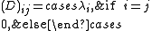
For each eigenvalue, λi, we have a specific eigenvalue equation
There will be 1 ≤ mi ≤ ni linearly independent solutions to each eigenvalue equation. The mi solutions are the eigenvectors associated with the eigenvalue λi. The integer mi is termed the geometric multiplicity of λi. It is important to keep in mind that the algebraic multiplicity ni and geometric multiplicity mi may or may not be equal, but we always have mi ≤ ni. The simplest case is of course when mi = ni = 1. The total number of linearly independent eigenvectors, Nv, can be calculated by summing the geometric multiplicities
The eigenvectors can be indexed by eigenvalues, i.e. using a double index, with vi,j being the jth eigenvector for the ith eigenvalue. The eigenvectors can also be indexed using the simpler notation of a single index vk, with k = 1, 2, ... , Nv.
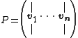
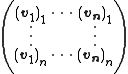
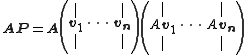
 Then A can be factorized
as
where Q is the square (N×N) matrix whose ith column is the eigenvector of A and Λ is the diagonal matrix
whose diagonal elements are the corresponding eigenvalues, i.e., . Note that only diagonalizable matrices
can be factorized in this way. For example, the matrix cannot be diagonalized.
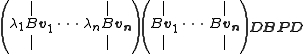
The eigenvectors are usually normalized, but they need not be. A non-normalized set of eigenvectors,
  can also be used as the columns of Q. That this is true can be understood by noting that the magnitude of the eigenvectors in Q gets canceled in the decomposition by the presence of Q−1.
Because Λ is a diagonal matrix
, its inverse is easy to calculate:
, the inverse
may be less valid when all eigenvalues are used unmodified in the form above. This is because as eigenvalues become relatively small, their contribution to the inversion is large. Those near zero or at the "noise" of the measurement system will have undue influence and could hamper solutions (detection) using the inverse.
Two mitigations have been proposed: 1) truncating small/zero eigenvalues, 2) extending the lowest reliable eigenvalue to those below it.
The first mitigation method is similar to a sparse sample of the original matrix, removing components that are not considered valuable. However, if the solution or detection process is near the noise level, truncating may remove components that influence the desired solution.
The second mitigation extends the eigenvalue so that lower values have much less influence over inversion, but do still contribute, such that solutions near the noise will still be found.
The reliable eigenvalue can be found by assuming that eigenvalues of extremely similar and low value are a good representation of measurement noise (which is assumed low for most systems).
If the eigenvalues are rank-sorted by value, then the reliable eigenvalue can be found by minimization of the Laplacian
of the sorted eigenvalues:

where the eigenvalues are subscripted with an 's' to denote being sorted. The position of the minimization is the lowest reliable eigenvalue. In measurement systems, the square root of this reliable eigenvalue is the average noise over the components of the system.
then we know that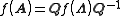
Because Λ is a diagonal matrix
, functions of Λ are very easy to calculate: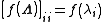
The off-diagonal elements of f(Λ) are zero; that is, f(Λ) is also a diagonal matrix. Therefore, calculating f(A) reduces to just calculating the function on each of the eigenvalues .
A similar technique works more generally with the holomorphic functional calculus
, using
from above. Once again, we find that


where Q is an orthonormal matrix, and Λ is a diagonal matrix whose entries are exactly the eigenvalues of A.
has an orthogonal eigenvector basis, so a normal matrix can be decomposed as
where U is a unitary matrix. Further, if A is Hermitian (which implies that it is also complex normal), the diagonal matrix Λ has only real values, and if A is unitary, Λ takes all its values on the complex unit circle.
Note that each eigenvalue is raised to the power ni, the algebraic multiplicity.
Note that each eigenvalue is multiplied by ni, the algebraic multiplicity.
. However, this is often impossible for larger matrices, in which case we must use a numerical method
.
In practice, eigenvalues of large matrices are not computed using the characteristic polynomial. Computing the polynomial becomes expensive in itself, and exact (symbolic) roots of a high-degree polynomial can be difficult to compute and express: the Abel–Ruffini theorem
implies that the roots of high-degree (5 and above) polynomials cannot in general be expressed simply using nth roots. Therefore, general algorithms to find eigenvectors and eigenvalues are iterative
.
Iterative numerical algorithms for approximating roots of polynomials exist, such as Newton's method
, but in general it is impractical to compute the characteristic polynomial and then apply these methods. One reason is that small round-off error
s in the coefficients of the characteristic polynomial can lead to large errors in the eigenvalues and eigenvectors: the roots are an extremely ill-conditioned function of the coefficients.
A simple and accurate iterative method is the power method: a random vector is chosen and a sequence of unit vectors is computed as
This sequence
will almost always
converge to an eigenvector corresponding to the eigenvalue of greatest magnitude, provided that v has a nonzero component of this eigenvector in the eigenvector basis (and also provided that there is only one eigenvalue of greatest magnitude)). This simple algorithm is useful in some practical applications; for example, Google
uses it to calculate the page rank
of documents in their search engine. Also, the power method is the starting point for many more sophisticated algorithms. For instance, by keeping not just the last vector in the sequence, but instead looking at the span
of all the vectors in the sequence, one can get a better (faster converging) approximation for the eigenvector, and this idea is the basis of Arnoldi iteration
. Alternatively, the important QR algorithm
is also based on a subtle transformation of a power method.
using Gaussian elimination
or any other method for solving matrix equations.
However, in practical large-scale eigenvalue methods, the eigenvectors are usually computed in other ways, as a byproduct of the eigenvalue computation. In power iteration
, for example, the eigenvector is actually computed before the eigenvalue (which is typically computed by the Rayleigh quotient of the eigenvector). In the QR algorithm for a Hermitian matrix (or any normal matrix
), the orthonormal eigenvectors are obtained as a product of the Q matrices from the steps in the algorithm. (For more general matrices, the QR algorithm yields the Schur decomposition
first, from which the eigenvectors can be obtained by a backsubstitution procedure.) For Hermitian matrices, the Divide-and-conquer eigenvalue algorithm
is more efficient than the QR algorithm if both eigenvectors and eigenvalues are desired.
This usage should not be confused with the generalized eigenvalue problem described below.
For example, in coherent electromagnetic scattering theory, the linear transformation A represents the action performed by the scattering object, and the eigenvectors represent polarization states of the electromagnetic wave. In optics
, the coordinate system is defined from the wave's viewpoint, known as the Forward Scattering Alignment
(FSA), and gives rise to a regular eigenvalue equation, whereas in radar
, the coordinate system is defined from the radar's viewpoint, known as the Back Scattering Alignment
(BSA), and gives rise to a coneigenvalue equation.
where A and B are matrices. If v obeys this equation, with some λ, then we call v the generalized eigenvector of A and B (in the 2nd sense), and λ is called the generalized eigenvalue of A and B (in the 2nd sense) which corresponds to the generalized eigenvector v.
The possible values of λ must obey the following equation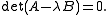
In the case we can find linearly independent vectors
 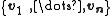 so that for every
  ,
,  , where
 then we define the matrices P and D such that
≡
Then the following equality holds
And the proof is
And since P is invertible, we multiply the equation from the right by its inverse and QED.
The set of matrices of the form , where
  is a complex number, is called a pencil; the term matrix pencil can also refer to the pair (A,B) of matrices.
If B is invertible, then the original problem can be written in the form
which is a standard eigenvalue problem. However, in most situations it is preferable not to perform the inversion, but rather to solve the generalized eigenvalue problem as stated originally. This is especially important if A and B are Hermitian matrices, since in this case is not generally Hermitian and important properties of the solution are no longer apparent.
If A and B are Hermitian and B is a positive-definite matrix
, the eigenvalues λ are real and eigenvectors v1 and v2 with distinct eigenvalues are B-orthogonal ( ). Also, in this case it is guaranteed that there exists a basis
of generalized eigenvectors (it is not a defective
problem). This case is sometimes called a Hermitian definite pencil or definite pencil.
Mathematics
Mathematics is the study of quantity, space, structure, and change. Mathematicians seek out patterns and formulate new conjectures. Mathematicians resolve the truth or falsity of conjectures by mathematical proofs, which are arguments sufficient to convince other mathematicians of their validity...
discipline of linear algebra
Linear algebra
Linear algebra is a branch of mathematics that studies vector spaces, also called linear spaces, along with linear functions that input one vector and output another. Such functions are called linear maps and can be represented by matrices if a basis is given. Thus matrix theory is often...
, eigendecomposition or sometimes spectral decomposition is the factorization
Factorization
In mathematics, factorization or factoring is the decomposition of an object into a product of other objects, or factors, which when multiplied together give the original...
of a matrix into a canonical form
Canonical form
Generally, in mathematics, a canonical form of an object is a standard way of presenting that object....
, whereby the matrix is represented in terms of its eigenvalues and eigenvectors. Only diagonalizable matrices
Diagonalizable matrix
In linear algebra, a square matrix A is called diagonalizable if it is similar to a diagonal matrix, i.e., if there exists an invertible matrix P such that P −1AP is a diagonal matrix...
can be factorized in this way.
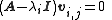
Fundamental theory of matrix eigenvectors and eigenvalues
A (non-zero) vector v of dimension N is an eigenvector of a square (N×N) matrix A if and only ifIf and only if
In logic and related fields such as mathematics and philosophy, if and only if is a biconditional logical connective between statements....
it satisfies the linear equation
where λ is a scalar, termed the eigenvalue corresponding to v. That is, the eigenvectors are the vectors which the linear transformation A merely elongates or shrinks, and the amount that they elongate/shrink by is the eigenvalue. The above equation is called the eigenvalue equation or the eigenvalue problem.
This yields an equation for the eigenvalues
We call p(λ) the characteristic polynomial
Characteristic polynomial
In linear algebra, one associates a polynomial to every square matrix: its characteristic polynomial. This polynomial encodes several important properties of the matrix, most notably its eigenvalues, its determinant and its trace....
, and the equation, called the characteristic equation, is an Nth order polynomial equation in the unknown λ. This equation will have Nλ distinct solutions, where 1 ≤ Nλ ≤ N . The set of solutions, i.e. the eigenvalues, is sometimes called the spectrum of A.
We can factor
Factorization
In mathematics, factorization or factoring is the decomposition of an object into a product of other objects, or factors, which when multiplied together give the original...
p as
The integer ni is termed the algebraic multiplicity of eigenvalue λi. The algebraic multiplicities sum to N:
For each eigenvalue, λi, we have a specific eigenvalue equation
There will be 1 ≤ mi ≤ ni linearly independent solutions to each eigenvalue equation. The mi solutions are the eigenvectors associated with the eigenvalue λi. The integer mi is termed the geometric multiplicity of λi. It is important to keep in mind that the algebraic multiplicity ni and geometric multiplicity mi may or may not be equal, but we always have mi ≤ ni. The simplest case is of course when mi = ni = 1. The total number of linearly independent eigenvectors, Nv, can be calculated by summing the geometric multiplicities
The eigenvectors can be indexed by eigenvalues, i.e. using a double index, with vi,j being the jth eigenvector for the ith eigenvalue. The eigenvectors can also be indexed using the simpler notation of a single index vk, with k = 1, 2, ... , Nv.
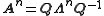
Eigendecomposition of a matrix
Let A be a square (N×N) matrix with N linearly independent eigenvectors, Then A can be factorizedMatrix decomposition
In the mathematical discipline of linear algebra, a matrix decomposition is a factorization of a matrix into some canonical form. There are many different matrix decompositions; each finds use among a particular class of problems.- Example :...
as
where Q is the square (N×N) matrix whose ith column is the eigenvector
of A and Λ is the diagonal matrixDiagonal matrix
In linear algebra, a diagonal matrix is a matrix in which the entries outside the main diagonal are all zero. The diagonal entries themselves may or may not be zero...
whose diagonal elements are the corresponding eigenvalues, i.e.,
. Note that only diagonalizable matricesDiagonalizable matrix
In linear algebra, a square matrix A is called diagonalizable if it is similar to a diagonal matrix, i.e., if there exists an invertible matrix P such that P −1AP is a diagonal matrix...
can be factorized in this way. For example, the matrix
cannot be diagonalized.The eigenvectors
are usually normalized, but they need not be. A non-normalized set of eigenvectors, can also be used as the columns of Q. That this is true can be understood by noting that the magnitude of the eigenvectors in Q gets canceled in the decomposition by the presence of Q−1.Matrix inverse via eigendecomposition
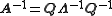
If matrix A can be eigendecomposed and if none of its eigenvalues are zero, then A is nonsingular and its inverse is given byBecause Λ is a diagonal matrix
Diagonal matrix
In linear algebra, a diagonal matrix is a matrix in which the entries outside the main diagonal are all zero. The diagonal entries themselves may or may not be zero...
, its inverse is easy to calculate:
Practical implications
When eigendecomposition is used on a matrix of measured, real dataData
The term data refers to qualitative or quantitative attributes of a variable or set of variables. Data are typically the results of measurements and can be the basis of graphs, images, or observations of a set of variables. Data are often viewed as the lowest level of abstraction from which...
, the inverse
Inverse function
In mathematics, an inverse function is a function that undoes another function: If an input x into the function ƒ produces an output y, then putting y into the inverse function g produces the output x, and vice versa. i.e., ƒ=y, and g=x...
may be less valid when all eigenvalues are used unmodified in the form above. This is because as eigenvalues become relatively small, their contribution to the inversion is large. Those near zero or at the "noise" of the measurement system will have undue influence and could hamper solutions (detection) using the inverse.
Two mitigations have been proposed: 1) truncating small/zero eigenvalues, 2) extending the lowest reliable eigenvalue to those below it.
The first mitigation method is similar to a sparse sample of the original matrix, removing components that are not considered valuable. However, if the solution or detection process is near the noise level, truncating may remove components that influence the desired solution.
The second mitigation extends the eigenvalue so that lower values have much less influence over inversion, but do still contribute, such that solutions near the noise will still be found.
The reliable eigenvalue can be found by assuming that eigenvalues of extremely similar and low value are a good representation of measurement noise (which is assumed low for most systems).
If the eigenvalues are rank-sorted by value, then the reliable eigenvalue can be found by minimization of the Laplacian
Laplace operator
In mathematics the Laplace operator or Laplacian is a differential operator given by the divergence of the gradient of a function on Euclidean space. It is usually denoted by the symbols ∇·∇, ∇2 or Δ...
of the sorted eigenvalues:
where the eigenvalues are subscripted with an 's' to denote being sorted. The position of the minimization is the lowest reliable eigenvalue. In measurement systems, the square root of this reliable eigenvalue is the average noise over the components of the system.
Functional calculus
The eigendecomposition allows for much easier computation of power series of matrices. If f(x) is given bythen we know that
Because Λ is a diagonal matrix
Diagonal matrix
In linear algebra, a diagonal matrix is a matrix in which the entries outside the main diagonal are all zero. The diagonal entries themselves may or may not be zero...
, functions of Λ are very easy to calculate:
The off-diagonal elements of f(Λ) are zero; that is, f(Λ) is also a diagonal matrix. Therefore, calculating f(A) reduces to just calculating the function on each of the eigenvalues .
A similar technique works more generally with the holomorphic functional calculus
Holomorphic functional calculus
In mathematics, holomorphic functional calculus is functional calculus with holomorphic functions. That is to say, given a holomorphic function ƒ of a complex argument z and an operator T, the aim is to construct an operatorf\,...
, using
from above. Once again, we find that
Examples
Symmetric matrices
Every N×N real nonsingular symmetric matrix has N linearly independent real eigenvectors. Moreover, these eigenvectors can be chosen such that they are orthogonal to each other and have norm one. Thus a real symmetric matrix A can be decomposed aswhere Q is an orthonormal matrix, and Λ is a diagonal matrix whose entries are exactly the eigenvalues of A.
Normal matrices
Similarly, a complex normal matrixNormal matrix
A complex square matrix A is a normal matrix ifA^*A=AA^* \ where A* is the conjugate transpose of A. That is, a matrix is normal if it commutes with its conjugate transpose.If A is a real matrix, then A*=AT...
has an orthogonal eigenvector basis, so a normal matrix can be decomposed as
where U is a unitary matrix. Further, if A is Hermitian (which implies that it is also complex normal), the diagonal matrix Λ has only real values, and if A is unitary, Λ takes all its values on the complex unit circle.
Useful facts regarding eigenvalues
- The product of the eigenvalues is equal to the determinantDeterminantIn linear algebra, the determinant is a value associated with a square matrix. It can be computed from the entries of the matrix by a specific arithmetic expression, while other ways to determine its value exist as well...
of A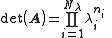
Note that each eigenvalue is raised to the power ni, the algebraic multiplicity.
- The sum of the eigenvalues is equal to the traceTrace (linear algebra)In linear algebra, the trace of an n-by-n square matrix A is defined to be the sum of the elements on the main diagonal of A, i.e.,...
of A
Note that each eigenvalue is multiplied by ni, the algebraic multiplicity.
- If the eigenvalues of A are λi, and A is invertible, then the eigenvalues of A-1 are simply λi−1.
- If the eigenvalues of A are λi, then the eigenvalues of f(A) are simply f(λi), for any holomorphic functionHolomorphic functionIn mathematics, holomorphic functions are the central objects of study in complex analysis. A holomorphic function is a complex-valued function of one or more complex variables that is complex differentiable in a neighborhood of every point in its domain...
f.
Useful facts regarding eigenvectors
- If A is (real) symmetric, then Nv = N, the eigenvectors are real, mutually orthogonal and provide a basis for
 .
. - The eigenvectors of A−1 are the same as the eigenvectors of A
- The eigenvectors of f(A) are the same as the eigenvectors of A
Useful facts regarding eigendecomposition
- A can be eigendecomposed if and only if

- If p(λ) has no repeated roots, i.e. Nλ = N, then A can be eigendecomposed.
- The statement "A can be eigendecomposed" does not imply that A has an inverse.
- The statement "A has an inverse" does not imply that A can be eigendecomposed.
Useful facts regarding matrix inverse
 can be inverted if and only if
- If
 and
and  , the inverse is given by
Numerical computation of eigenvalues
Suppose that we want to compute the eigenvalues of a given matrix. If the matrix is small, we can compute them symbolically using the characteristic polynomialCharacteristic polynomial
In linear algebra, one associates a polynomial to every square matrix: its characteristic polynomial. This polynomial encodes several important properties of the matrix, most notably its eigenvalues, its determinant and its trace....
. However, this is often impossible for larger matrices, in which case we must use a numerical method
Numerical analysis
Numerical analysis is the study of algorithms that use numerical approximation for the problems of mathematical analysis ....
.
In practice, eigenvalues of large matrices are not computed using the characteristic polynomial. Computing the polynomial becomes expensive in itself, and exact (symbolic) roots of a high-degree polynomial can be difficult to compute and express: the Abel–Ruffini theorem
Abel–Ruffini theorem
In algebra, the Abel–Ruffini theorem states that there is no general algebraic solution—that is, solution in radicals— to polynomial equations of degree five or higher.- Interpretation :...
implies that the roots of high-degree (5 and above) polynomials cannot in general be expressed simply using nth roots. Therefore, general algorithms to find eigenvectors and eigenvalues are iterative
Iterative method
In computational mathematics, an iterative method is a mathematical procedure that generates a sequence of improving approximate solutions for a class of problems. A specific implementation of an iterative method, including the termination criteria, is an algorithm of the iterative method...
.
Iterative numerical algorithms for approximating roots of polynomials exist, such as Newton's method
Newton's method
In numerical analysis, Newton's method , named after Isaac Newton and Joseph Raphson, is a method for finding successively better approximations to the roots of a real-valued function. The algorithm is first in the class of Householder's methods, succeeded by Halley's method...
, but in general it is impractical to compute the characteristic polynomial and then apply these methods. One reason is that small round-off error
Round-off error
A round-off error, also called rounding error, is the difference between the calculated approximation of a number and its exact mathematical value. Numerical analysis specifically tries to estimate this error when using approximation equations and/or algorithms, especially when using finitely many...
s in the coefficients of the characteristic polynomial can lead to large errors in the eigenvalues and eigenvectors: the roots are an extremely ill-conditioned function of the coefficients.
A simple and accurate iterative method is the power method: a random vector
is chosen and a sequence of unit vectors is computed as
This sequence
Sequence
In mathematics, a sequence is an ordered list of objects . Like a set, it contains members , and the number of terms is called the length of the sequence. Unlike a set, order matters, and exactly the same elements can appear multiple times at different positions in the sequence...
will almost always
Almost Always
"Almost Always" is a popular song. It was recorded by Joni James in 1953. The recording was released by MGM as catalog number 11470. The song was only on the Billboard magazine charts for one week, reaching #18 on May 9, 1953. The flip side was "Is It Any Wonder?"...
converge to an eigenvector corresponding to the eigenvalue of greatest magnitude, provided that v has a nonzero component of this eigenvector in the eigenvector basis (and also provided that there is only one eigenvalue of greatest magnitude)). This simple algorithm is useful in some practical applications; for example, Google
Google
Google Inc. is an American multinational public corporation invested in Internet search, cloud computing, and advertising technologies. Google hosts and develops a number of Internet-based services and products, and generates profit primarily from advertising through its AdWords program...
uses it to calculate the page rank
PageRank
PageRank is a link analysis algorithm, named after Larry Page and used by the Google Internet search engine, that assigns a numerical weighting to each element of a hyperlinked set of documents, such as the World Wide Web, with the purpose of "measuring" its relative importance within the set...
of documents in their search engine. Also, the power method is the starting point for many more sophisticated algorithms. For instance, by keeping not just the last vector in the sequence, but instead looking at the span
Linear span
In the mathematical subfield of linear algebra, the linear span of a set of vectors in a vector space is the intersection of all subspaces containing that set...
of all the vectors in the sequence, one can get a better (faster converging) approximation for the eigenvector, and this idea is the basis of Arnoldi iteration
Arnoldi iteration
In numerical linear algebra, the Arnoldi iteration is an eigenvalue algorithm and an important example of iterative methods. Arnoldi finds the eigenvalues of general matrices; an analogous method for Hermitian matrices is the Lanczos iteration. The Arnoldi iteration was invented by W. E...
. Alternatively, the important QR algorithm
QR algorithm
In numerical linear algebra, the QR algorithm is an eigenvalue algorithm: that is, a procedure to calculate the eigenvalues and eigenvectors of a matrix. The QR transformation was developed in the late 1950s by John G.F. Francis and by Vera N. Kublanovskaya , working independently...
is also based on a subtle transformation of a power method.
Numerical computation of eigenvectors
Once the eigenvalues are computed, the eigenvectors could be calculated by solving the equationusing Gaussian elimination
Gaussian elimination
In linear algebra, Gaussian elimination is an algorithm for solving systems of linear equations. It can also be used to find the rank of a matrix, to calculate the determinant of a matrix, and to calculate the inverse of an invertible square matrix...
or any other method for solving matrix equations.
However, in practical large-scale eigenvalue methods, the eigenvectors are usually computed in other ways, as a byproduct of the eigenvalue computation. In power iteration
Power iteration
In mathematics, the power iteration is an eigenvalue algorithm: given a matrix A, the algorithm will produce a number λ and a nonzero vector v , such that Av = λv....
, for example, the eigenvector is actually computed before the eigenvalue (which is typically computed by the Rayleigh quotient of the eigenvector). In the QR algorithm for a Hermitian matrix (or any normal matrix
Normal matrix
A complex square matrix A is a normal matrix ifA^*A=AA^* \ where A* is the conjugate transpose of A. That is, a matrix is normal if it commutes with its conjugate transpose.If A is a real matrix, then A*=AT...
), the orthonormal eigenvectors are obtained as a product of the Q matrices from the steps in the algorithm. (For more general matrices, the QR algorithm yields the Schur decomposition
Schur decomposition
In the mathematical discipline of linear algebra, the Schur decomposition or Schur triangulation, named after Issai Schur, is a matrix decomposition.- Statement :...
first, from which the eigenvectors can be obtained by a backsubstitution procedure.) For Hermitian matrices, the Divide-and-conquer eigenvalue algorithm
Divide-and-conquer eigenvalue algorithm
Divide-and-conquer eigenvalue algorithms are a class of eigenvalue algorithms for Hermitian or real symmetric matrices that have recently become competitive in terms of stability and efficiency with more traditional algorithms such as the QR algorithm. The basic concept behind these algorithms is...
is more efficient than the QR algorithm if both eigenvectors and eigenvalues are desired.
Generalized eigenspaces
Recall that the geometric multiplicity of an eigenvalue can be described as the dimension of the associated eigenspace, the nullspace of λI − A. The algebraic multiplicity can also be thought of as a dimension: it is the dimension of the associated generalized eigenspace (1st sense), which is the nullspace of the matrix (λI − A)k for any sufficiently large k. That is, it is the space of generalized eigenvectors (1st sense), where a generalized eigenvector is any vector which eventually becomes 0 if λI − A is applied to it enough times successively. Any eigenvector is a generalized eigenvector, and so each eigenspace is contained in the associated generalized eigenspace. This provides an easy proof that the geometric multiplicity is always less than or equal to the algebraic multiplicity.This usage should not be confused with the generalized eigenvalue problem described below.
Conjugate eigenvector
A conjugate eigenvector or coneigenvector is a vector sent after transformation to a scalar multiple of its conjugate, where the scalar is called the conjugate eigenvalue or coneigenvalue of the linear transformation. The coneigenvectors and coneigenvalues represent essentially the same information and meaning as the regular eigenvectors and eigenvalues, but arise when an alternative coordinate system is used. The corresponding equation is
For example, in coherent electromagnetic scattering theory, the linear transformation A represents the action performed by the scattering object, and the eigenvectors represent polarization states of the electromagnetic wave. In optics
Optics
Optics is the branch of physics which involves the behavior and properties of light, including its interactions with matter and the construction of instruments that use or detect it. Optics usually describes the behavior of visible, ultraviolet, and infrared light...
, the coordinate system is defined from the wave's viewpoint, known as the Forward Scattering Alignment
Forward scattering alignment
The Forward Scattering Alignment is a coordinate system used in coherent electromagnetic scattering.The coordinate system is defined from the viewpoint of the electromagnetic wave, before and after scattering...
(FSA), and gives rise to a regular eigenvalue equation, whereas in radar
Radar
Radar is an object-detection system which uses radio waves to determine the range, altitude, direction, or speed of objects. It can be used to detect aircraft, ships, spacecraft, guided missiles, motor vehicles, weather formations, and terrain. The radar dish or antenna transmits pulses of radio...
, the coordinate system is defined from the radar's viewpoint, known as the Back Scattering Alignment
Back scattering alignment
The Back Scattering Alignment is a coordinate system used in coherent electromagnetic scattering. The coordinate system is defined from the viewpoint of the wave source, before and after scattering. The BSA is most commonly used in radar, specifically when working with a Sinclair Matrix because...
(BSA), and gives rise to a coneigenvalue equation.
Generalized eigenvalue problem
A generalized eigenvalue problem (2nd sense) is the problem of finding a vector v that obeys
where A and B are matrices. If v obeys this equation, with some λ, then we call v the generalized eigenvector of A and B (in the 2nd sense), and λ is called the generalized eigenvalue of A and B (in the 2nd sense) which corresponds to the generalized eigenvector v.
The possible values of λ must obey the following equation
In the case we can find
linearly independent vectors so that for every , , where then we define the matrices P and D such that≡
Then the following equality holds
And the proof is
And since P is invertible, we multiply the equation from the right by its inverse and QED.
The set of matrices of the form
, where is a complex number, is called a pencil; the term matrix pencil can also refer to the pair (A,B) of matrices.If B is invertible, then the original problem can be written in the form

which is a standard eigenvalue problem. However, in most situations it is preferable not to perform the inversion, but rather to solve the generalized eigenvalue problem as stated originally. This is especially important if A and B are Hermitian matrices, since in this case
is not generally Hermitian and important properties of the solution are no longer apparent.If A and B are Hermitian and B is a positive-definite matrix
Positive-definite matrix
In linear algebra, a positive-definite matrix is a matrix that in many ways is analogous to a positive real number. The notion is closely related to a positive-definite symmetric bilinear form ....
, the eigenvalues λ are real and eigenvectors v1 and v2 with distinct eigenvalues are B-orthogonal (
). Also, in this case it is guaranteed that there exists a basisBasis (linear algebra)
In linear algebra, a basis is a set of linearly independent vectors that, in a linear combination, can represent every vector in a given vector space or free module, or, more simply put, which define a "coordinate system"...
of generalized eigenvectors (it is not a defective
Defective matrix
In linear algebra, a defective matrix is a square matrix that does not have a complete basis of eigenvectors, and is therefore not diagonalizable. In particular, an n × n matrix is defective if and only if it does not have n linearly independent eigenvectors...
problem). This case is sometimes called a Hermitian definite pencil or definite pencil.
See also
- Matrix decompositionMatrix decompositionIn the mathematical discipline of linear algebra, a matrix decomposition is a factorization of a matrix into some canonical form. There are many different matrix decompositions; each finds use among a particular class of problems.- Example :...
- List of matrices
- Eigenvalue, eigenvector and eigenspaceEigenvalue, eigenvector and eigenspaceThe eigenvectors of a square matrix are the non-zero vectors that, after being multiplied by the matrix, remain parallel to the original vector. For each eigenvector, the corresponding eigenvalue is the factor by which the eigenvector is scaled when multiplied by the matrix...
- Spectral theoremSpectral theoremIn mathematics, particularly linear algebra and functional analysis, the spectral theorem is any of a number of results about linear operators or about matrices. In broad terms the spectral theorem provides conditions under which an operator or a matrix can be diagonalized...
- Householder transformationHouseholder transformationIn linear algebra, a Householder transformation is a linear transformation that describes a reflection about a plane or hyperplane containing the origin. Householder transformations are widely used in numerical linear algebra, to perform QR decompositions and in the first step of the QR algorithm...