Lagrange multipliers - AbsoluteAstronomy.com

In mathematical optimization, the method of Lagrange multipliers (named after Joseph Louis Lagrange

Joseph Louis Lagrange

Joseph-Louis Lagrange , born Giuseppe Lodovico Lagrangia, was a mathematician and astronomer, who was born in Turin, Piedmont, lived part of his life in Prussia and part in France, making significant contributions to all fields of analysis, to number theory, and to classical and celestial mechanics...

) provides a strategy for finding the maxima and minima of a function

Function (mathematics)

In mathematics, a function associates one quantity, the argument of the function, also known as the input, with another quantity, the value of the function, also known as the output. A function assigns exactly one output to each input. The argument and the value may be real numbers, but they can...

subject to constraints

Constraint (mathematics)

In mathematics, a constraint is a condition that a solution to an optimization problem must satisfy. There are two types of constraints: equality constraints and inequality constraints...

.

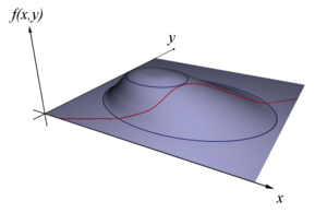
For instance (see Figure 1), consider the optimization problem

maximize

subject to

We introduce a new variable (

) called a Lagrange multiplier, and study the Lagrange function defined by

where the

may be either positive or negative. If

is a maximum for the original constrained problem, then there exists

such that

is a stationary point

Stationary point

In mathematics, particularly in calculus, a stationary point is an input to a function where the derivative is zero : where the function "stops" increasing or decreasing ....

for the Lagrange function (stationary points are those points where the partial derivatives of Λ are zero). However, not all stationary points yield a solution of the original problem. Thus, the method of Lagrange multipliers yields a necessary condition for optimality in constrained problems.

Introduction

Consider the two-dimensional problem introduced above:

maximize

subject to

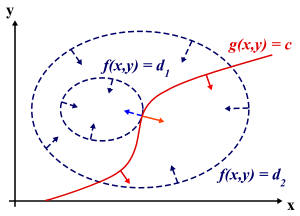
We can visualize contour

Contour line

A contour line of a function of two variables is a curve along which the function has a constant value. In cartography, a contour line joins points of equal elevation above a given level, such as mean sea level...

s of f given by

for various values of

, and the contour of

given by

.

Suppose we walk along the contour line with

. In general the contour lines of

and

may be distinct, so following the contour line for

one could intersect with or cross the contour lines of

. This is equivalent to saying that while moving along the contour line for

the value of

can vary. Only when the contour line for

meets contour lines of

tangentially

Contact (mathematics)

In mathematics, contact of order k of functions is an equivalence relation, corresponding to having the same value at a point P and also the same derivatives there, up to order k. The equivalence classes are generally called jets...

, do we not increase or decrease the value of

— that is, when the contour lines touch but do not cross.

The contour lines of f and g touch when the tangent vectors of the contour lines are parallel. Since the gradient

Gradient

In vector calculus, the gradient of a scalar field is a vector field that points in the direction of the greatest rate of increase of the scalar field, and whose magnitude is the greatest rate of change....

of a function is perpendicular to the contour lines, this is the same as saying that the gradients of f and g are parallel. Thus we want points

where

and

,
where

and

are the respective gradients. The constant

is required because although the two gradient vectors are parallel, the magnitudes of the gradient vectors are generally not equal.

To incorporate these conditions into one equation, we introduce an auxiliary function

and solve

This is the method of Lagrange multipliers. Note that

implies

Not necessarily extrema

The constrained extrema of

are critical points
Critical point (mathematics)
In calculus, a critical point of a function of a real variable is any value in the domain where either the function is not differentiable or its derivative is 0. The value of the function at a critical point is a critical value of the function...

of the Lagrangian

, but they are not local extrema of

(see Example 2 below).

One may reformulate the Lagrangian as a Hamiltonian

Hamiltonian mechanics

Hamiltonian mechanics is a reformulation of classical mechanics that was introduced in 1833 by Irish mathematician William Rowan Hamilton.It arose from Lagrangian mechanics, a previous reformulation of classical mechanics introduced by Joseph Louis Lagrange in 1788, but can be formulated without...

, in which case the solutions are local minima for the Hamiltonian. This is done in optimal control

Optimal control

Optimal control theory, an extension of the calculus of variations, is a mathematical optimization method for deriving control policies. The method is largely due to the work of Lev Pontryagin and his collaborators in the Soviet Union and Richard Bellman in the United States.-General method:Optimal...

theory, in the form of Pontryagin's minimum principle

Pontryagin's minimum principle

Pontryagin's maximum principle is used in optimal control theory to find the best possible control for taking a dynamical system from one state to another, especially in the presence of constraints for the state or input controls. It was formulated by the Russian mathematician Lev Semenovich...

.

The fact that solutions of the Lagrangian are not necessarily extrema also poses difficulties for numerical optimization. This can be addressed by computing the magnitude of the gradient, as the zeros of the magnitude are necessarily local minima, as illustrated in the numerical optimization example.

Handling multiple constraints

The method of Lagrange multipliers can also accommodate multiple constraints. To see how this is done, we need to reexamine the problem in a
slightly different manner because the concept of “crossing” discussed above becomes rapidly unclear when we consider the types of constraints
that are created when we have more than one constraint acting together.

As an example, consider a paraboloid

Paraboloid

In mathematics, a paraboloid is a quadric surface of special kind. There are two kinds of paraboloids: elliptic and hyperbolic. The elliptic paraboloid is shaped like an oval cup and can have a maximum or minimum point....

with a constraint that is a single point (as might be created if we had 2 line constraints
that intersect). The level set

Level set

In mathematics, a level set of a real-valued function f of n variables is a set of the formthat is, a set where the function takes on a given constant value c....

(i.e., contour line) clearly appears to “cross” that point and its gradient

Gradient

is clearly not parallel
to the gradients of either of the two line constraints. Yet, it is obviously a maximum and a minimum because there is only one point
on the paraboloid that meets the constraint.

While this example seems a bit odd, it is easy to understand and is representative of the sort of “effective” constraint that appears
quite often when we deal with multiple constraints intersecting. Thus, we take a slightly different approach below to explain and derive
the Lagrange Multipliers method with any number of constraints.

Throughout this section, the independent variables will be denoted by

and, as a group,
we will denote them as

. Also, the function being analyzed will be denoted
by

and the constraints will be represented by the equations

.

The basic idea remains essentially the same: if we consider only the points that satisfy the constraints (i.e. are in the constraints),
then a point

is a stationary point (i.e. a point in a “flat” region) of f if
and only if the constraints at that point do not allow movement in a direction where f changes value.

Once we have located the stationary points, we need to do further tests to see if we have found a minimum, a maximum or just a stationary
point that is neither.

We start by considering the level set of f at

. The set of vectors

containing the directions in which we can move and still remain in the same level set are the
directions where the value of f does not change (i.e. the change equals zero). Thus, for every vector
v in

, the following relation must hold:

where the notation

above means the

-component of the vector v.
The equation above can be rewritten in a more compact geometric form that helps our intuition:

This makes it clear that if we are at p, then all directions from this point that do not change the value of
f must be perpendicular to

(the gradient of f at p).

Now let us consider the effect of the constraints. Each constraint limits the directions that we can move from a particular point
and still satisfy the constraint. We can use the same procedure, to look for the set of vectors

containing the directions in which we can move and still satisfy the constraint. As above, for every vector
v in

, the following relation must hold:

From this, we see that at point p, all directions from this point that will still satisfy this constraint must be
perpendicular to

.

Now we are ready to refine our idea further and complete the method: a point on f is a constrained stationary point if and only if the direction that changes f violates at least one of the constraints. (We can see that this is true because if a
direction that changes f did not violate any constraints, then there would a “legal” point nearby with a higher or lower
value for f and the current point would then not be a stationary point.)

Single constraint revisited

For a single constraint, we use the statement above to say that at stationary points the direction that changes f is in the same direction
that violates the constraint. To determine if two vectors are in the same direction, we note that if two vectors start from the same
point and are “in the same direction”, then one vector can always “reach” the other by changing its length and/or flipping to point the
opposite way along the same direction line. In this way, we can succinctly state that two vectors point in the same direction if and
only if one of them can be multiplied by some real number such that they become equal to the other. So, for our purposes, we require that:

If we now add another simultaneous equation to guarantee that we only perform this test when we are at a point that satisfies the
constraint, we end up with 2 simultaneous equations that when solved, identify all constrained stationary points:

Note that the above is a succinct way of writing the equations. Fully expanded, there are

simultaneous equations that need to be
solved for the

variables which are

and

Multiple constraints

For more than one constraint, the same reasoning applies. If there is more than one constraint active together, each constraint
contributes a direction that will violate it. Together, these “violation directions” form a “violation space”, where infinitesimal
movement in any direction within the space will violate one or more constraints. Thus, to satisfy multiple constraints we can state
(using this new terminology) that at the stationary points, the direction that changes f is in the “violation space” created by the
constraints acting jointly.

The violation space created by the constraints consists of all points that can be reached by adding any combination of scaled
and/or flipped versions of the individual violation direction vectors. In other words, all the points that are “reachable” when
we use the individual violation directions as the basis of the space. Thus, we can succinctly state that v is in the space defined
by

if and only if there exists a set of “multipliers”

such that:

which for our purposes, translates to stating that the direction that changes f at p is in the “violation space” defined by the
constraints

if and only if:

As before, we now add simultaneous equation to guarantee that we only perform this test when we are at a point that satisfies every
constraint, we end up with simultaneous equations that when solved, identify all constrained stationary points:

The method is complete now (from the standpoint of solving the problem of finding stationary points) but as mathematicians delight in
doing, these equations can be further condensed into an even more elegant and succinct form. Lagrange must have cleverly noticed that
the equations above look like partial derivatives of some larger scalar function L that takes all the

and all the

as inputs. Next, he might then have noticed that setting every equation equal to zero is exactly what one would have to do to solve for the unconstrained
stationary points of that larger function. Finally, he showed that a larger function L with partial derivatives that are exactly the ones we require can be constructed very simply as below:

Solving the equation above for its unconstrained stationary points generates exactly the same stationary points as solving for the
constrained stationary points of f under the constraints

.

In Lagrange’s honor, the function above is called a Lagrangian, the scalars

are called Lagrange Multipliers and this optimization method itself is called The Method of Lagrange Multipliers.

The method of Lagrange multipliers is generalized by the Karush–Kuhn–Tucker conditions, which can also take into account inequality constraints of the form h(x) ≤ c.

Interpretation of the Lagrange multipliers

Often the Lagrange multipliers have an interpretation as some quantity of interest. To see why
this might be the case, observe that:

So, λ_k is the rate of change of the quantity being optimized as a function of the constraint variable.
As examples, in Lagrangian mechanics

Lagrangian mechanics

Lagrangian mechanics is a re-formulation of classical mechanics that combines conservation of momentum with conservation of energy. It was introduced by the Italian-French mathematician Joseph-Louis Lagrange in 1788....

the equations of motion are derived by finding stationary points of the action

Action (physics)

In physics, action is an attribute of the dynamics of a physical system. It is a mathematical functional which takes the trajectory, also called path or history, of the system as its argument and has a real number as its result. Action has the dimension of energy × time, and its unit is...

, the time integral of the difference between kinetic and potential energy. Thus, the force on a particle due to a scalar potential,

, can be interpreted as a Lagrange multiplier determining the change in action (transfer of potential to kinetic energy) following a variation in the particle's constrained trajectory. In economics, the optimal profit to a player is calculated subject to a constrained space of actions, where a Lagrange multiplier is the increase in the value of the objective function due to the relaxation of a given constraint (e.g. through an increase in income or bribery or other means) – the marginal cost

Marginal cost

In economics and finance, marginal cost is the change in total cost that arises when the quantity produced changes by one unit. That is, it is the cost of producing one more unit of a good...

of a constraint, called the shadow price

Shadow price

In constrained optimization in economics, the shadow price is the instantaneous change per unit of the constraint in the objective value of the optimal solution of an optimization problem obtained by relaxing the constraint...

.

In control theory this is formulated instead as costate equations.

Example 1

Suppose one wishes to maximize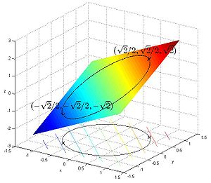

subject to the constraint

. The feasible set is the unit circle, and the level set

Level set

In mathematics, a level set of a real-valued function f of n variables is a set of the formthat is, a set where the function takes on a given constant value c....

s of f are diagonal lines (with slope -1), so one can see graphically that the maximum occurs at

, and the minimum occurs at

.

Formally, set

, and

Set the derivative

, which yields the system of equations:

As always, the

equation ((iii) here) is the original constraint.

Combining the first two equations yields

(explicitly,

, otherwise (i) yields 1 = 0, so one has

).

Substituting into (iii) yields

, so

and

, showing the stationary points are

and

. Evaluating the objective function f on these yields

thus the maximum is

, which is attained at

, and the minimum is

, which is attained at

Example 2

Suppose one wants to find the maximum values of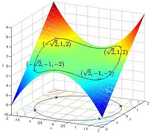

with the condition that the x and y coordinates lie on the circle around the origin with radius √3, that is, subject to the constraint

As there is just a single constraint, we will use only one multiplier, say λ.

The constraint g(x, y)-3 is identically zero on the circle of radius √3. So any multiple of g(x, y)-3 may be added to f(x, y) leaving f(x, y) unchanged in the region of interest (above the circle where our original constraint is satisfied). Let

The critical values of

occur where its gradient is zero. The partial derivatives are

Equation (iii) is just the original constraint. Equation (i) implies

or λ = −y. In the first case, if x = 0 then we must have

by (iii) and then by (ii) λ = 0. In the second case, if λ = −y and substituting into equation (ii) we have that,

Then x² = 2y². Substituting into equation (iii) and solving for y gives this value of y:

Thus there are six critical points:

Evaluating the objective at these points, we find

Therefore, the objective function attains the global maximum (subject to the constraints) at

and the global minimum at

The point

is a local minimum and

is a local maximum, as may be determined by consideration of the Hessian matrix of

.

Note that while

is a critical point of

, it is not a local extremum. We have

. Given any neighborhood of

, we can choose a small positive

and a small

of either sign to get

values both greater and less than

Example: entropy

Suppose we wish to find the discrete probability distribution on the points

with maximal information entropy

Information entropy

In information theory, entropy is a measure of the uncertainty associated with a random variable. In this context, the term usually refers to the Shannon entropy, which quantifies the expected value of the information contained in a message, usually in units such as bits...

. This is the same as saying that we wish to find the least biased

Bias of an estimator

In statistics, bias of an estimator is the difference between this estimator's expected value and the true value of the parameter being estimated. An estimator or decision rule with zero bias is called unbiased. Otherwise the estimator is said to be biased.In ordinary English, the term bias is...

probability distribution on the points

. In other words, we wish to maximize the Shannon entropy equation:

For this to be a probability distribution the sum of the probabilities

at each point

must equal 1, so our constraint is

= 1:

We use Lagrange multipliers to find the point of maximum entropy,

, across all discrete probability distributions

. We require that:

which gives a system of n equations,

, such that:

Carrying out the differentiation of these n equations, we get

This shows that all

are equal (because they depend on λ only).
By using the constraint ∑_j p_j = 1, we find

Hence, the uniform distribution is the distribution with the greatest entropy, among distributions on n points.

Example: numerical optimization

With Lagrange multipliers, the critical points occur at saddle point

Saddle point

In mathematics, a saddle point is a point in the domain of a function that is a stationary point but not a local extremum. The name derives from the fact that in two dimensions the surface resembles a saddle that curves up in one direction, and curves down in a different direction...

s, rather than at local maxima (or minima). Unfortunately, many numerical optimization techniques, such as hill climbing

Hill climbing

In computer science, hill climbing is a mathematical optimization technique which belongs to the family of local search. It is an iterative algorithm that starts with an arbitrary solution to a problem, then attempts to find a better solution by incrementally changing a single element of the solution...

, gradient descent

Gradient descent

Gradient descent is a first-order optimization algorithm. To find a local minimum of a function using gradient descent, one takes steps proportional to the negative of the gradient of the function at the current point...

, some of the quasi-Newton method

Quasi-Newton method

In optimization, quasi-Newton methods are algorithms for finding local maxima and minima of functions. Quasi-Newton methods are based on...

s, among others, are designed to find local maxima (or minima) and not saddle points. For this reason, one must either modify the formulation to ensure that it's a minimization problem (for example, by extremizing the square of the gradient

Gradient

of the Lagrangian as below), or else use an optimization technique that finds stationary points (such as Newton's method

Newton's method in optimization

In mathematics, Newton's method is an iterative method for finding roots of equations. More generally, Newton's method is used to find critical points of differentiable functions, which are the zeros of the derivative function.-Method:...

without an extremum seeking line search) and not necessarily extrema.

As a simple example, consider the problem of finding the value of x that minimizes

, constrained such that

. (This problem is somewhat pathological because there are only two values that satisfy this constraint, but it is useful for illustration purposes because the corresponding unconstrained function can be visualized in three dimensions.)

Using Lagrange multipliers, this problem can be converted into an unconstrained optimization problem:

The two critical points occur at saddle points where

and

.

In order to solve this problem with a numerical optimization technique, we must first transform this problem such that the critical points occur at local minima. This is done by computing the magnitude of the gradient of the unconstrained optimization problem.

First, we compute the partial derivative of the unconstrained problem with respect to each variable:

If the target function is not easily differentiable, the differential with respect to each variable can be approximated as

,

where

is a small value.

Next, we compute the magnitude of the gradient, which is the square root of the sum of the squares of the partial derivatives:

(Since magnitude is always non-negative, optimizing over the squared-magnitude is equivalent to optimizing over the magnitude. Thus, the ``square root" may be omitted from these equations with no expected difference in the results of optimization.)

The critical points of h occur at

and

, just as in

. Unlike the critical points in

, however, the critical points in h occur at local minima, so numerical optimization techniques can be used to find them.

Economics

Constrained optimization plays a central role in economics

Economics

Economics is the social science that analyzes the production, distribution, and consumption of goods and services. The term economics comes from the Ancient Greek from + , hence "rules of the house"...

. For example, the choice problem for a consumer

Consumer theory

Consumer choice is a theory of microeconomics that relates preferences for consumption goods and services to consumption expenditures and ultimately to consumer demand curves. The link between personal preferences, consumption, and the demand curve is one of the most closely studied relations in...

is represented as one of maximizing a utility function subject to a budget constraint

Budget constraint

A budget constraint represents the combinations of goods and services that a consumer can purchase given current prices with his or her income. Consumer theory uses the concepts of a budget constraint and a preference map to analyze consumer choices...

. The Lagrange multiplier has an economic interpretation as the shadow price

Shadow price

associated with the constraint, in this example the marginal utility

Marginal utility

In economics, the marginal utility of a good or service is the utility gained from an increase in the consumption of that good or service...

of income

Income

Income is the consumption and savings opportunity gained by an entity within a specified time frame, which is generally expressed in monetary terms. However, for households and individuals, "income is the sum of all the wages, salaries, profits, interests payments, rents and other forms of earnings...

Control theory

In optimal control

Optimal control

theory, the Lagrange multipliers are interpreted as costate variables, and Lagrange multipliers are reformulated as the minimization of the Hamiltonian

Hamiltonian mechanics

, in Pontryagin's minimum principle

Pontryagin's minimum principle

External links

Exposition

Conceptual introduction (plus a brief discussion of Lagrange multipliers in the calculus of variations
Calculus of variations
Calculus of variations is a field of mathematics that deals with extremizing functionals, as opposed to ordinary calculus which deals with functions. A functional is usually a mapping from a set of functions to the real numbers. Functionals are often formed as definite integrals involving unknown...

as used in physics)
Lagrange Multipliers for Quadratic Forms With Linear Constraints by Kenneth H. Carpenter

For additional text and interactive applets

Simple explanation with an example of governments using taxes as Lagrange multipliers
Applet
Tutorial and applet
Video Lecture of Lagrange Multipliers
MIT Video Lecture on Lagrange Multipliers
Slides accompanying Bertsekas's nonlinear optimization text, with details on Lagrange multipliers (lectures 11 and 12)
http://eom.springer.de/L/l057190.htm
Method of Lagrange multipliers with complex variables by kipid

The source of this article is wikipedia, the free encyclopedia. The text of this article is licensed under the GFDL.

Introduction

Not necessarily extrema

Handling multiple constraints

Single constraint revisited

Multiple constraints

Interpretation of the Lagrange multipliers

Example 1

Example 2

Example: entropy

Example: numerical optimization

Economics

Control theory

See also

External links