

Numerical smoothing and differentiation
Encyclopedia
An experimental datum value can be conceptually described as the sum of a signal and some noise
, but in practice the two contributions cannot be separated. The purpose of smoothing is to increase the Signal-to-noise ratio
without greatly distorting the signal (i.e. to get rid of the noise). One way to achieve this is by fitting successive sets of m data points to a polynomial
of degree less than m by the method of linear least squares
. Once the coefficients of the smoothing polynomial have been calculated they can be used to give estimates of the signal or its derivatives.
method of numerical smoothing and differentiation.
Suppose that the data consists of a set of n {xi, yi} points (i = 1...n), where x is an independent variable and yi is an observed value. A polynomial will be fitted to a set of m (an odd number) adjacent data points, each separated by an interval h. Firstly, a change of variable is made
where is the value of the central point. z takes the values (1-m)/2 .. 0 .. (m-1)/2 (e.g. m = 5 → z = [-2,-1,0,1,2]). The polynomial, of degree k is defined as
The coefficients a0, a1 etc. are obtained by solving the normal equations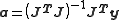
where the ith row of the Jacobian matrix J has the values {1 zi zi2 … zik}. For example, for a quadratic polynomial fitted to 5 points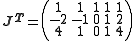
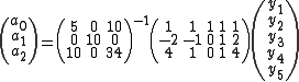
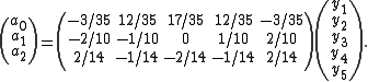
In this example, . This is the smoothed value for the central point (
 ) of the five data points used in the calculation.
The coefficients (-3 12 17 12 -3)/35 are known as convolution
coefficients as they are applied in succession to sets of m points at a time.
Tables of convolution coefficients were published by Savitzky and Golay
in 1964, though the procedure for calculating them was known in the 19th century (See E. T. Whittaker and G. Robinson, The Calculus of Observations)
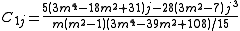
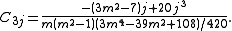
The numerical derivatives are obtained by differentiating Y. For a cubic polynomial
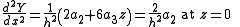

It is not necessary always to use the Savitzky-Golay tables as algebraic formulae can be derived for the convolution coefficients. For a cubic polynomial the expressions are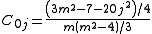
For example, If the noise in all data points has a constant Standard deviation
, σ, when smoothing by a m-point linear polynomial the standard deviation on the noise will be decreased to , but with a quadratic polynomial it reduces to approximately
  . So, for a 9-point quadratic smooth only half the noise is removed.
co-domain
(see pseudocode
below). The (finite) Fourier transform
of a convolution filter shows that it is most efficient for high-frequency noise and can therefore be described as a low-pass filter. The noise that is not removed is primarily low-frequency noise.
### Smooth the vector x[1,...,nx] with an exponentially damped kernel. The
### result is a vector "smooth" with indeterminate values at the edges, and
### smoothed values in between
cutoff = 0.05 ### weights to zero below this value
alpha = 1.8 ### Decay of weight with distance from center
logacutoff = log(cutoff)/log(alpha) ### log base alpha of cutoff
span = floor(-logacutoff ) ### width to left and right
weights = alpha^(-abs(sequence(left=-span, right=span, step=1))) ### Overloaded "^"
kernel = weights / sum(weights) ### Overloaded "/"
nx = length(x)
nk = 2*span+1 ### length(kernel)
assert( nx>nk )
x1 = concatenate( sequence(0,length=ny-1), x )
k1 = concatenate( kernel, sequence(0,length=nx-1) )
s1 = inverse_fft( fft(x1) * fft(k1) ) ### Overloaded "*"
smooth = sequence(NaN, length=nx)
smooth[1+span:nx-span] = s1[ ny+nk-1 : nx+nk-1 ] ### using 1 offset notation
Noise
In common use, the word noise means any unwanted sound. In both analog and digital electronics, noise is random unwanted perturbation to a wanted signal; it is called noise as a generalisation of the acoustic noise heard when listening to a weak radio transmission with significant electrical noise...
, but in practice the two contributions cannot be separated. The purpose of smoothing is to increase the Signal-to-noise ratio
Signal-to-noise ratio
Signal-to-noise ratio is a measure used in science and engineering that compares the level of a desired signal to the level of background noise. It is defined as the ratio of signal power to the noise power. A ratio higher than 1:1 indicates more signal than noise...
without greatly distorting the signal (i.e. to get rid of the noise). One way to achieve this is by fitting successive sets of m data points to a polynomial
Polynomial
In mathematics, a polynomial is an expression of finite length constructed from variables and constants, using only the operations of addition, subtraction, multiplication, and non-negative integer exponents...
of degree less than m by the method of linear least squares
Linear least squares
In statistics and mathematics, linear least squares is an approach to fitting a mathematical or statistical model to data in cases where the idealized value provided by the model for any data point is expressed linearly in terms of the unknown parameters of the model...
. Once the coefficients of the smoothing polynomial have been calculated they can be used to give estimates of the signal or its derivatives.
Convolution coefficients
When the data points are equally spaced a relatively simple analytical solution to the least-squares equations can be found. This solution forms the basis of the convolutionConvolution
In mathematics and, in particular, functional analysis, convolution is a mathematical operation on two functions f and g, producing a third function that is typically viewed as a modified version of one of the original functions. Convolution is similar to cross-correlation...
method of numerical smoothing and differentiation.
Suppose that the data consists of a set of n {xi, yi} points (i = 1...n), where x is an independent variable and yi is an observed value. A polynomial will be fitted to a set of m (an odd number) adjacent data points, each separated by an interval h. Firstly, a change of variable is made
where
is the value of the central point. z takes the values (1-m)/2 .. 0 .. (m-1)/2 (e.g. m = 5 → z = [-2,-1,0,1,2]). The polynomial, of degree k is defined asThe coefficients a0, a1 etc. are obtained by solving the normal equations
where the ith row of the Jacobian matrix J has the values {1 zi zi2 … zik}. For example, for a quadratic polynomial fitted to 5 points
In this example,
. This is the smoothed value for the central point () of the five data points used in the calculation.The coefficients (-3 12 17 12 -3)/35 are known as convolution
Convolution
In mathematics and, in particular, functional analysis, convolution is a mathematical operation on two functions f and g, producing a third function that is typically viewed as a modified version of one of the original functions. Convolution is similar to cross-correlation...
coefficients as they are applied in succession to sets of m points at a time.
Tables of convolution coefficients were published by Savitzky and Golay
Savitzky–Golay smoothing filter
The Savitzky–Golay smoothing filter is a type of filter first described in 1964 by Abraham Savitzky and Marcel J. E. Golay.The Savitzky–Golay method essentially performs a local polynomial regression on a series of values to determine the smoothed value for each point...
in 1964, though the procedure for calculating them was known in the 19th century (See E. T. Whittaker and G. Robinson, The Calculus of Observations)
The numerical derivatives are obtained by differentiating Y. For a cubic polynomial
It is not necessary always to use the Savitzky-Golay tables as algebraic formulae can be derived for the convolution coefficients. For a cubic polynomial the expressions are
Signal distortion and noise reduction
It is inevitable that the signal will be distorted in the convolution process. Both the extent of the distortion and signal-to-noise improvement:- decrease as the degree of the polynomial increases
- increase as the width, m of the convolution function increases
For example, If the noise in all data points has a constant Standard deviation
Standard deviation
Standard deviation is a widely used measure of variability or diversity used in statistics and probability theory. It shows how much variation or "dispersion" there is from the average...
, σ, when smoothing by a m-point linear polynomial the standard deviation on the noise will be decreased to
, but with a quadratic polynomial it reduces to approximately . So, for a 9-point quadratic smooth only half the noise is removed.Frequency characteristics of convolution filters
Convolution maps to multiplication in the FourierFourier
Fourier most commonly refers to Joseph Fourier , French mathematician and physicist, or the mathematics, physics, and engineering terms named in his honor for his work on the concepts underlying them:In mathematics:...
co-domain
Codomain
In mathematics, the codomain or target set of a function is the set into which all of the output of the function is constrained to fall. It is the set in the notation...
(see pseudocode
Pseudocode
In computer science and numerical computation, pseudocode is a compact and informal high-level description of the operating principle of a computer program or other algorithm. It uses the structural conventions of a programming language, but is intended for human reading rather than machine reading...
below). The (finite) Fourier transform
Fourier transform
In mathematics, Fourier analysis is a subject area which grew from the study of Fourier series. The subject began with the study of the way general functions may be represented by sums of simpler trigonometric functions...
of a convolution filter shows that it is most efficient for high-frequency noise and can therefore be described as a low-pass filter. The noise that is not removed is primarily low-frequency noise.
### Smooth the vector x[1,...,nx] with an exponentially damped kernel. The
### result is a vector "smooth" with indeterminate values at the edges, and
### smoothed values in between
cutoff = 0.05 ### weights to zero below this value
alpha = 1.8 ### Decay of weight with distance from center
logacutoff = log(cutoff)/log(alpha) ### log base alpha of cutoff
span = floor(-logacutoff ) ### width to left and right
weights = alpha^(-abs(sequence(left=-span, right=span, step=1))) ### Overloaded "^"
kernel = weights / sum(weights) ### Overloaded "/"
nx = length(x)
nk = 2*span+1 ### length(kernel)
assert( nx>nk )
x1 = concatenate( sequence(0,length=ny-1), x )
k1 = concatenate( kernel, sequence(0,length=nx-1) )
s1 = inverse_fft( fft(x1) * fft(k1) ) ### Overloaded "*"
smooth = sequence(NaN, length=nx)
smooth[1+span:nx-span] = s1[ ny+nk-1 : nx+nk-1 ] ### using 1 offset notation
Applications
- Smoothing by convolution is performed primarily for aesthetic reasons. Fitting statistical models to smoothed data is generally a mistake, since the smoothing process alters the distribution of noise.
- Location of maxima and minimaMaxima and minimaIn mathematics, the maximum and minimum of a function, known collectively as extrema , are the largest and smallest value that the function takes at a point either within a given neighborhood or on the function domain in its entirety .More generally, the...
in experimental data curves. The first derivative of a function is zero at a maximum or minimum. - Location of an end-point in a titration curveTitration curveTitrations are often recorded on titration curves, whose compositions are generally identical: the independent variable is the volume of the titrant, while the dependent variable is the pH of the solution...
. An end-point is an inflection pointInflection pointIn differential calculus, an inflection point, point of inflection, or inflection is a point on a curve at which the curvature or concavity changes sign. The curve changes from being concave upwards to concave downwards , or vice versa...
where the second derivative of the function is zero. - Resolution enhancement in spectroscopy. Bands in the second derivative of a spectroscopic curve are narrower than the bands in the spectrum: they have reduced Half-widthFull width at half maximumFull width at half maximum is an expression of the extent of a function, given by the difference between the two extreme values of the independent variable at which the dependent variable is equal to half of its maximum value....
. This allows partially overlapping bands to be "resolved" into separate peaks.
External links
- Savitsky-Golay filter (in Dutch, but with good illustrations)
- Savitsky-Golay/Low-noise Lanczos differentiators Derivation, reference formulas, study on noise suppression properties in frequency domain.
- Smooth noise-robust differentiation Alternative approach to differentiate noisy data/function.