
Nonuniform rational B-spline
Encyclopedia
B-spline
In the mathematical subfield of numerical analysis, a B-spline is a spline function that has minimal support with respect to a given degree, smoothness, and domain partition. B-splines were investigated as early as the nineteenth century by Nikolai Lobachevsky...
(NURBS) is a mathematical model commonly used in computer graphics
Computer graphics
Computer graphics are graphics created using computers and, more generally, the representation and manipulation of image data by a computer with help from specialized software and hardware....
for generating and representing curves and surfaces which offers great flexibility and precision for handling both analytic (shapes defined by common mathematical formulas) and freeform shapes.
History
Development of NURBS began in the 1950s by engineers who were in need of a mathematically precise representation of freeform surfaces like those used for ship hulls, aerospace exterior surfaces, and car bodies, which could be exactly reproduced whenever technically needed. Prior representations of this kind of surface only existed as a single physical model created by a designerDesigner
A designer is a person who designs. More formally, a designer is an agent that "specifies the structural properties of a design object". In practice, anyone who creates tangible or intangible objects, such as consumer products, processes, laws, games and graphics, is referred to as a...
.
The pioneers of this development were Pierre Bézier
Pierre Bézier
Pierre Étienne Bézier was a French engineer and one of the founders of the fields of solid, geometric and physical modeling as well as in the field of representing curves, especially in CAD/CAM systems...
who worked as an engineer at Renault
Renault
Renault S.A. is a French automaker producing cars, vans, and in the past, autorail vehicles, trucks, tractors, vans and also buses/coaches. Its alliance with Nissan makes it the world's third largest automaker...
, and Paul de Casteljau
Paul de Casteljau
Paul de Casteljau is a French physicist and mathematician. In 1959, while working at Citroën, he developed an algorithm for computation of Bézier curves, which would later be formalized and popularized by engineer Pierre Bézier...
who worked at Citroën
Citroën
Citroën is a major French automobile manufacturer, part of the PSA Peugeot Citroën group.Founded in 1919 by French industrialist André-Gustave Citroën , Citroën was the first mass-production car company outside the USA and pioneered the modern concept of creating a sales and services network that...
, both in France
France
The French Republic , The French Republic , The French Republic , (commonly known as France , is a unitary semi-presidential republic in Western Europe with several overseas territories and islands located on other continents and in the Indian, Pacific, and Atlantic oceans. Metropolitan France...
. Bézier worked nearly parallel to de Casteljau, neither knowing about the work of the other. But because Bézier published the results of his work, the average computer graphics
Computer graphics
Computer graphics are graphics created using computers and, more generally, the representation and manipulation of image data by a computer with help from specialized software and hardware....
user today recognizes spline
Spline (mathematics)
In mathematics, a spline is a sufficiently smooth piecewise-polynomial function. In interpolating problems, spline interpolation is often preferred to polynomial interpolation because it yields similar results, even when using low-degree polynomials, while avoiding Runge's phenomenon for higher...
s — which are represented with control points lying off the curve itself — as Bézier spline
Bézier spline
In the mathematical field of numerical analysis and in computer graphics, a Bézier spline is a spline curve where each polynomial of the spline is in Bézier form....
s, while de Casteljau’s name is only known and used for the algorithms he developed to evaluate parametric surface
Parametric surface
A parametric surface is a surface in the Euclidean space R3 which is defined by a parametric equation with two parameters. Parametric representation is the most general way to specify a surface. Surfaces that occur in two of the main theorems of vector calculus, Stokes' theorem and the divergence...
s. In the 1960s it became clear that non-uniform, rational B-splines are a generalization
Generalization
A generalization of a concept is an extension of the concept to less-specific criteria. It is a foundational element of logic and human reasoning. Generalizations posit the existence of a domain or set of elements, as well as one or more common characteristics shared by those elements. As such, it...
of Bézier splines, which can be regarded as uniform, non-rational B-splines.
At first NURBS were only used in the proprietary CAD packages of car companies. Later they became part of standard computer graphics packages.
Real-time, interactive rendering of NURBS curves and surfaces was first made available on Silicon Graphics
Silicon Graphics
Silicon Graphics, Inc. was a manufacturer of high-performance computing solutions, including computer hardware and software, founded in 1981 by Jim Clark...
workstations in 1989. In 1993, the first interactive NURBS modeller for PCs, called NöRBS, was developed by CAS Berlin, a small startup company cooperating with the Technical University of Berlin. Today most professional computer graphics applications available for desktop use offer NURBS technology, which is most often realized by integrating a NURBS engine from a specialized company.
Use
Computer-aided manufacturing
Computer-aided manufacturing is the use of computer software to control machine tools and related machinery in the manufacturing of workpieces. This is not the only definition for CAM, but it is the most common; CAM may also refer to the use of a computer to assist in all operations of a...
), and engineering (CAE
Computer-aided engineering
Computer-aided engineering is the broad usage of computer software to aid in engineering tasks. It includes computer-aided design , computer-aided analysis , computer-integrated manufacturing , computer-aided manufacturing , material requirements planning , and computer-aided planning .- Overview...
) and are part of numerous industry wide used standards, such as IGES
IGES
The Initial Graphics Exchange Specification is a file format which defines a vendor neutral data format that allows the digital exchange of information among Computer-aided design systems....
, STEP
ISO 10303
ISO 10303 is an ISO standard for the computer-interpretable representation and exchange of product manufacturing information. Its official title is: Automation systems and integration — Product data representation and exchange...
, ACIS
ACIS
The 3D ACIS Modeler is a 3D modelling kernel owned by Spatial Corporation . ACIS is used by many software developers in industries such as computer-aided design , Computer-aided manufacturing , Computer-aided engineering , Architecture, engineering and construction , Coordinate-measuring machine...
, and PHIGS
PHIGS
PHIGS is an API standard for rendering 3D computer graphics, at one time considered to be the 3D graphics standard for the 1990s. Instead a combination of features and power led to the rise of OpenGL, which became the most popular professional 3D API of the 1990s...
. NURBS tools are also found in various 3D modeling and animation
Animation
Animation is the rapid display of a sequence of images of 2-D or 3-D artwork or model positions in order to create an illusion of movement. The effect is an optical illusion of motion due to the phenomenon of persistence of vision, and can be created and demonstrated in several ways...
software packages, such as form•Z
Form-Z
form·Z is a computer-aided design tool developed by AutoDesSys for all design fields that deal with the articulation of 3D spaces and forms and which is used for 3D modeling, drafting, animation and rendering.-Overview:...
, Blender
Blender (software)
Blender is a free and open-source 3D computer graphics software product used for creating animated films, visual effects, interactive 3D applications or video games. The current release version is 2.60, and was released on October 19, 2011...
,3ds Max, Maya
Maya (software)
Autodesk Maya , commonly shortened to Maya, is 3D computer graphics software that runs on Microsoft Windows, Mac OS and Linux, originally developed by Alias Systems Corporation and currently owned and developed by Autodesk, Inc. It is used to create interactive 3D applications, including video...
, Rhino3D, Cinema 4D
Cinema 4D
CINEMA 4D is a 3D modeling, animation and rendering application developed by MAXON Computer GmbH of Friedrichsdorf, Germany. It is capable of procedural and polygonal/subd modeling, animating, lighting, texturing, rendering, and common features found in 3d modelling applications.- Overview:The...
, Cobalt
Cobalt (CAD program)
Cobalt is a parametric-based computer-aided design and 3D modeling program that runs on both Macintosh and Microsoft Windows operating systems...
, Shark FX, and Solid Modeling Solutions. Other than this there are specialized NURBS modeling software packages such as Autodesk Alias Surface
Autodesk Alias Surface
Alias Software is a division of Autodesk which publishes software used in automotive styling.The software allows to create 2D sketches and rendering and it features the use of modern Cintique Tablets. This digital workflow opens an entire new world of image creation...
, solidThinking
SolidThinking
solidThinking is a 3D modeling and rendering software, developed by solidThinking Inc. It is a CAID software, i.e...
and ICEM Surf.
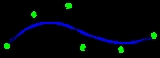
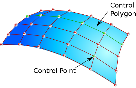
They allow representation of geometrical shapes in a compact form. They can be efficiently handled by the computer programs and yet allow for easy human interaction. NURBS surfaces are functions of two parameters mapping to a surface in three-dimensional space. The shape of the surface is determined by control points.
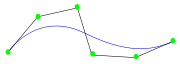
In general, editing NURBS curves and surfaces is highly intuitive and predictable. Control points are always either connected directly to the curve/surface, or act as if they were connected by a rubber band. Depending on the type of user interface, editing can be realized via an element’s control points, which are most obvious and common for Bézier curve
Bézier curve
A Bézier curve is a parametric curve frequently used in computer graphics and related fields. Generalizations of Bézier curves to higher dimensions are called Bézier surfaces, of which the Bézier triangle is a special case....
s, or via higher level tools such as spline modeling or hierarchical editing.
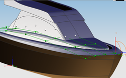
A surface under construction, e.g. the hull of a motor yacht, is usually composed of several NURBS surfaces known as patches. These patches should be fitted together in
such a way that the boundaries are invisible. This is mathematically expressed by the concept of geometric continuity.
Higher-level tools exist which benefit from the ability of NURBS to create and establish geometric continuity of different levels:
Positional continuity (G0): holds whenever the end positions of two curves or surfaces are coincidental. The curves or surfaces may still meet at an angle, giving rise to a sharp corner or edge and causing broken highlights.
Tangential continuity (G1): requires the end vectors of the curves or surfaces to be parallel, ruling out sharp edges. Because highlights falling on a tangentially continuous edge are always continuous and thus look natural, this level of continuity can often be sufficient.
Curvature continuity (G2): further requires the end vectors to be of the same length and rate of length change. Highlights falling on a curvature-continuous edge do not display any change, causing the two surfaces to appear as one. This can be visually recognized as “perfectly smooth”. This level of continuity is very useful in the creation of models that require many bi-cubic patches composing one continuous surface.
Geometric continuity mainly refers to the shape of the resulting surface; since NURBS surfaces are functions, it is also possible to discuss the derivatives of the surface with respect to the parameters. This is known as parametric continuity. Parametric continuity of a given degree implies geometric continuity of that degree.
First- and second-level parametric continuity (C0 and C1) are for practical purposes identical to positional and tangential (G0 and G1) continuity. Third-level parametric continuity (C2), however, differs from curvature continuity in that its parameterization is also continuous. In practice, C2 continuity is easier to achieve if uniform B-splines are used.
The definition of the continuity 'Cn requires that the nth derivative of the curve/surface (
 ) are equal at a joint. Note that the (partial) derivatives of curves and surfaces are vectors that have a direction and a magnitude. Both should be equal.
Highlights and reflections can reveal the perfect smoothing, which is otherwise practically impossible to achieve without NURBS surfaces that have at least G2 continuity. This same principle is used as one of the surface evaluation methods whereby a ray-traced or reflection-mapped
Reflection mapping
In computer graphics, environment mapping, or reflection mapping, is an efficient Image-based lighting technique for approximating the appearance of a reflective surface by means of a precomputed texture image. The texture is used to store the image of the distant environment surrounding the...
image of a surface with white stripes reflecting on it will show even the smallest deviations on a surface or set of surfaces. This method is derived from car prototyping wherein surface quality is inspected by checking the quality of reflections of a neon-light ceiling on the car surface. This method is also known as "Zebra analysis".
Technical specifications
A NURBS curve is defined by its order, a set of weighted control points, and a knot vector. NURBS curves and surfaces are generalizations of both B-splineB-spline
In the mathematical subfield of numerical analysis, a B-spline is a spline function that has minimal support with respect to a given degree, smoothness, and domain partition. B-splines were investigated as early as the nineteenth century by Nikolai Lobachevsky...
s and Bézier curve
Bézier curve
A Bézier curve is a parametric curve frequently used in computer graphics and related fields. Generalizations of Bézier curves to higher dimensions are called Bézier surfaces, of which the Bézier triangle is a special case....
s and surfaces, the primary difference being the weighting of the control points which makes NURBS curves rational (non-rational B-splines are a special case of rational B-splines).
Whereas Bézier curves evolve into only one parametric direction, usually called s or u, NURBS surfaces evolve into two parametric directions, called s and t or u and v.
NURBS curves and surfaces are useful for a number of reasons:
- They are invariantInvariant (mathematics)In mathematics, an invariant is a property of a class of mathematical objects that remains unchanged when transformations of a certain type are applied to the objects. The particular class of objects and type of transformations are usually indicated by the context in which the term is used...
under affineAffine transformationIn geometry, an affine transformation or affine map or an affinity is a transformation which preserves straight lines. It is the most general class of transformations with this property...
as well as perspectiveGraphical projectionGraphical projection is a protocol by which an image of a three-dimensional object is projected onto a planar surface without the aid of mathematical calculation, used in technical drawing.- Overview :...
transformations: operations like rotations and translations can be applied to NURBS curves and surfaces by applying them to their control points. - They offer one common mathematical form for both standard analytical shapes (e.g., conics) and free-form shapes.
- They provide the flexibility to design a large variety of shapes.
- They reduce the memory consumption when storing shapes (compared to simpler methods).
- They can be evaluated reasonably quickly by numerically stable and accurate algorithmAlgorithmIn mathematics and computer science, an algorithm is an effective method expressed as a finite list of well-defined instructions for calculating a function. Algorithms are used for calculation, data processing, and automated reasoning...
s.
In the next sections, NURBS is discussed in one dimension (curves). It should be noted that all of it can be generalized to two or even more dimensions.
Control points
The control points determine the shape of the curve. Typically, each point of the curve is computed by taking a weighted sum of a number of control points. The weight of each point varies according to the governing parameter. For a curve of degree d, the weight of any control point is only nonzero in d+1 intervals of the parameter space. Within those intervals, the weight changes according to a polynomial function (basis functions) of degree d. At the boundaries of the intervals, the basis functions go smoothly to zero, the smoothness being determined by the degree of the polynomial.As an example, the basis function of degree one is a triangle function. It rises from zero to one, then falls to zero again. While it rises, the basis function of the previous control point falls. In that way, the curve interpolates between the two points, and the resulting curve is a polygon, which is continuous
Continuous function
In mathematics, a continuous function is a function for which, intuitively, "small" changes in the input result in "small" changes in the output. Otherwise, a function is said to be "discontinuous". A continuous function with a continuous inverse function is called "bicontinuous".Continuity of...
, but not differentiable at the interval boundaries, or knots. Higher degree polynomials have correspondingly more continuous derivatives. Note that within the interval the polynomial nature of the basis functions and the linearity of the construction make the curve perfectly smooth, so it is only at the knots that discontinuity can arise.
The fact that a single control point only influences those intervals where it is active is a highly desirable property, known as local support. In modeling, it allows the changing of one part of a surface while keeping other parts equal.
Adding more control points allows better approximation to a given curve, although only a certain class of curves can be represented exactly with a finite number of control points. NURBS curves also feature a scalar weight for each control point. This allows for more control over the shape of the curve without unduly raising the number of control points. In particular, it adds conic sections like circles and ellipses to the set of curves that can be represented exactly. The term rational in NURBS refers to these weights.
The control points can have any dimensionality. One-dimensional points just define a scalar
Scalar (mathematics)
In linear algebra, real numbers are called scalars and relate to vectors in a vector space through the operation of scalar multiplication, in which a vector can be multiplied by a number to produce another vector....
function of the parameter. These are typically used in image processing programs to tune the brightness and color curves. Three-dimensional control points are used abundantly in 3D modeling, where they are used in the everyday meaning of the word 'point', a location in 3D space.
Multi-dimensional points might be used to control sets of time-driven values, e.g. the different positional and rotational settings of a robot arm. NURBS surfaces are just an application of this. Each control 'point' is actually a full vector of control points, defining a curve. These curves share their degree and the number of control points, and span one dimension of the parameter space. By interpolating these control vectors over the other dimension of the parameter space, a continuous set of curves is obtained, defining the surface.
The knot vector
The knot vector is a sequence of parameter values that determines where and how the control points affect the NURBS curve. The number of knots is always equal to the number of control points plus curve degree plus one. The knot vector divides the parametric space in the intervals mentioned before, usually referred to as knot spans. Each time the parameter value enters a new knot span, a new control point becomes active, while an old control point is discarded.It follows that the values in the knot vector should be in nondecreasing order, so (0, 0, 1, 2, 3, 3) is valid while (0, 0, 2, 1, 3, 3) is not.
Consecutive knots can have the same value. This then defines a knot span of zero length, which implies that two control points are activated at the same time (and of course two control points become deactivated). This has impact on continuity of the resulting curve or its higher derivatives; for instance, it allows the creation of corners in an otherwise smooth NURBS curve.
A number of coinciding knots is sometimes referred to as a knot with a certain multiplicity. Knots with multiplicity two or three are known as double or triple knots.
The multiplicity of a knot is limited to the degree of the curve; since a higher multiplicity would split the curve into disjoint parts and it would leave control points unused. For first-degree NURBS, each knot is paired with a control point.
The knot vector usually starts with a knot that has multiplicity equal to the order. This makes sense, since this activates the control points that have influence on the first knot span. Similarly, the knot vector usually ends with a knot of that multiplicity.
Curves with such knot vectors start and end in a control point.
The individual knot values are not meaningful by themselves; only the ratios of the difference between the knot values matter. Hence, the knot vectors (0, 0, 1, 2, 3, 3) and (0, 0, 2, 4, 6, 6) produce the same curve. The positions of the knot values influences the mapping of parameter space to curve space. Rendering a NURBS curve is usually done by stepping with a fixed stride through the parameter range. By changing the knot span lengths, more sample points can be used in regions where the curvature is high. Another use is in situations where the parameter value has some physical significance, for instance if the parameter is time and the curve describes the motion of a robot arm. The knot span lengths then translate into velocity and acceleration, which are essential to get right to prevent damage to the robot arm or its environment. This flexibility in the mapping is what the phrase non uniform in NURBS refers to.
Necessary only for internal calculations, knots are usually not helpful to the users of modeling software. Therefore, many modeling applications do not make the knots editable or even visible. It's usually possible to establish reasonable knot vectors by looking at the variation in the control points. More recent versions of NURBS software (e.g., Autodesk Maya and Rhinoceros 3D
Rhinoceros 3D
Rhinoceros is a stand-alone, commercial NURBS-based 3-D modeling tool, developed by Robert McNeel & Associates. The software is commonly used for industrial design, architecture, marine design, jewelry design, automotive design, CAD / CAM, rapid prototyping, reverse engineering as well as the...
) allow for interactive editing of knot positions, but this is significantly less intuitive than the editing of control points.
Order
The order of a NURBS curve defines the number of nearby control points that influence any given point on the curve. The curve is represented mathematically by a polynomial of degree one less than the order of the curve. Hence, second-order curves (which are represented by linear polynomials) are called linear curves, third-order curves are called quadratic curves, and fourth-order curves are called cubic curves. The number of control points must be greater than or equal to the order of the curve.In practice, cubic curves are the ones most commonly used. Fifth- and sixth-order curves are sometimes useful, especially for obtaining continuous higher order derivatives, but curves of higher orders are practically never used because they lead to internal numerical problems and tend to require disproportionately large calculation times.
Construction of the basis functions
The basis functions used in NURBS curves are usually denoted as , in which
  corresponds to the
  -th
-thcontrol point, and
 corresponds with the degree of the basis function. The parameter dependence is frequently left out, so we can write
  .
.The definition of these basis functions is recursive in
 .
.The degree-0 functions
 are piecewise constant functions. They are one on the corresponding knot span and zero everywhere else.
Effectively,
 is a linear interpolation of
  and
and  . The latter two functions are non-zero for
 knot spans, overlapping for
  knot spans. The function
  is computed as
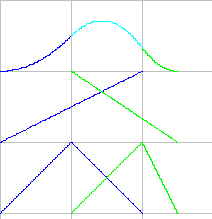

 rises linearly from zero to one on the interval where
  is non-zero, while
  falls from one to zero on the interval where
  is non-zero. As mentioned before,
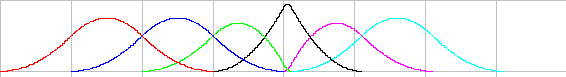
  is a triangular function, nonzero over two knot spans rising from zero to one on the first, and falling to zero on the second knot span. Higher order basis functions are non-zero over corresponding more knot spans and have correspondingly higher degree. If
  is the parameter, and
  is the
  -th knot, we can write the functions
  and
and  as
as
and

The functions
 and
and  are positive when the corresponding lower order basis functions are non-zero. By induction
Mathematical induction
Mathematical induction is a method of mathematical proof typically used to establish that a given statement is true of all natural numbers...
on n it follows that the basis functions are non-negative for all values of
 and
and  . This makes the computation of the basis functions numerically stable.
Again by induction, it can be proved that the sum of the basis functions for a particular value of the parameter is unity. This is known as the partition of unity property of the basis functions.
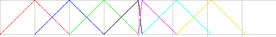
One knot span is considerably shorter than the others. On that knot span, the peak in the quadratic basis function is more distinct, reaching almost one. Conversely, the adjoining basis functions fall to zero more quickly. In the geometrical interpretation, this means that the curve approaches the corresponding control point closely. In case of a double knot, the length of the knot span becomes zero and the peak reaches one exactly. The basis function is no longer differentiable at that point. The curve will have a sharp corner if the neighbour control points are not collinear.
General form of a NURBS curve
Using the definitions of the basis functions from the previous paragraph, a NURBS curve takes the following form:
-

In this, is the number of control points
  and
and  are the corresponding weights. The denominator is a normalizing factor that evaluates to one if all weights are one. This can be seen from the partition of unity property of the basis functions. It is customary to write this as
in which the functions
are known as the rational basis functions.
Manipulating NURBS objects
A number of transformations can be applied to a NURBS object. For instance, if some curve is defined using a certain degree and N control points, the same curve can be expressed using the same degree and N+1 control points. In the process a number of control points change position and a knot is inserted in the knot vector.
These manipulations are used extensively during interactive design. When adding a control point, the shape of the curve should stay the same, forming the starting point for further adjustments. A number of these operations are discussed below.
Knot insertion
As the term suggests, knot insertion inserts a knot into the knot vector. If the degree of the curve is , then
  control points are replaced by
  new ones. The shape of the curve stays the same.
A knot can be inserted multiple times, up to the maximum multiplicity of the knot. This is sometimes referred to as knot refinement and can be achieved by an algorithm that is more efficient than repeated knot insertion.
Knot removal
Knot removal is the reverse of knot insertion. Its purpose is to remove knots and the associated control points in order to get a more compact representation. Obviously, this is not always possible while retaining the exact shape of the curve. In practice, a tolerance in the accuracy is used to determine whether a knot can be removed. The process is used to clean up after an interactive session in which control points may have been added manually, or after importing
a curve from a different representation, where a straightforward conversion process leads to redundant control points.
Degree elevation
A NURBS curve of a particular degree can always be represented by a NURBS curve of higher degree. This is frequently used when combining separate NURBS curves,
e.g. when creating a NURBS surface interpolating between a set of NURBS curves or when unifying adjacent curves. In the process, the different curves should be brought to the same degree, usually the maximum degree of the set of curves. The process is known as degree elevation.
Curvature
The most important property in differential geometry is the curvatureCurvatureIn mathematics, curvature refers to any of a number of loosely related concepts in different areas of geometry. Intuitively, curvature is the amount by which a geometric object deviates from being flat, or straight in the case of a line, but this is defined in different ways depending on the context...
 . It describes the local properties (edges, corners, etc.) and relations between the first and second derivative, and thus, the precise curve shape. Having determined the derivatives it is easy to compute
  or approximated as the arclength from the second derivate
  . The direct computation of the curvature
  with these equations is the big advantage of parameterized curves against their polygonal representations.
Example: a circle
Non-rational splines or Bézier curveBézier curveA Bézier curve is a parametric curve frequently used in computer graphics and related fields. Generalizations of Bézier curves to higher dimensions are called Bézier surfaces, of which the Bézier triangle is a special case....
s may approximate a circle, but they cannot represent it exactly. Rational splines can represent any conic section, including the circle, exactly. This representation is not unique, but one possibility appears below:
x y z weight 1 0 0 1 1 1 0 
0 1 0 1 −1 1 0 
−1 0 0 1 −1 −1 0 
0 −1 0 1 1 −1 0 
1 0 0 1
The order is two, since a circle is a quadratic curve and the spline's order is one more than the degree of its piecewise polynomial segments. The knot vector is . The circle is composed of four quarter circles, tied together with double knots. Although double knots in a third order NURBS curve would normally result in loss of continuity in the first derivative, the control points are positioned in such a way that the first derivative is continuous. (In fact, the curve is infinitely differentiable everywhere, as it must be if it exactly represents a circle.)
The curve represents a circle exactly, but it is not exactly parametrized in the circle's arc length. This means, for example, that the point at does not lie at
  (except for the start, middle and end point of each quarter circle, since the representation is symmetrical). This is obvious; the x coordinate of the circle would otherwise provide an exact rational polynomial expression for
  , which is impossible. The circle does make one full revolution as its parameter
  goes from 0 to
  , but this is only because the knot vector was arbitrarily chosen as multiples of
  .
.
See also
- SplineSpline (mathematics)In mathematics, a spline is a sufficiently smooth piecewise-polynomial function. In interpolating problems, spline interpolation is often preferred to polynomial interpolation because it yields similar results, even when using low-degree polynomials, while avoiding Runge's phenomenon for higher...
- Bézier surfaceBézier surfaceBézier surfaces are a species of mathematical spline used in computer graphics, computer-aided design, and finite element modeling.As with the Bézier curve, a Bézier surface is defined by a set of control points...
- de Boor's algorithmDe Boor's algorithmIn the mathematical subfield of numerical analysis the de Boor's algorithm is a fast and numerically stable algorithm for evaluating spline curves in B-spline form. It is a generalization of the de Casteljau's algorithm for Bézier curves. The algorithm was devised by Carl R. de Boor...
- Subdivision surfaceSubdivision surfaceA subdivision surface, in the field of 3D computer graphics, is a method of representing a smooth surface via the specification of a coarser piecewise linear polygon mesh...
- Triangle meshTriangle meshA triangle mesh is a type of polygon mesh in computer graphics. It comprises a set of triangles that are connected by their common edges or corners....
- Point cloudPoint cloudA point cloud is a set of vertices in a three-dimensional coordinate system. These vertices are usually defined by X, Y, and Z coordinates, and typically are intended to be representative of the external surface of an object....
- Rational motionRational motionIn kinematics, the motion of a rigid body is defined as a continuous set of displacements. One-parameter motions can be definedas a continuous displacement of moving object with respect to a fixed frame in Euclidean three-space , where the displacement depends on one parameter, mostly identified as...
- Isogeometric analysisIsogeometric AnalysisIsogeometric analysis is a recently developed computational approach that offers the possibility of integrating finite element analysis into conventional NURBS-based CAD design tools. Currently, it is necessary to convert data between CAD and FEA packages to analyse new designs during development,...
External links
- About Nonuniform Rational B-Splines - NURBS
- An Interactive Introduction to Splines
- http://www.cs.bris.ac.uk/Teaching/Resources/COMS30115/all.pdf
- http://homepages.inf.ed.ac.uk/rbf/CVonline/LOCAL_COPIES/AV0405/DONAVANIK/bezier.html
- http://mathcs.holycross.edu/~croyden/csci343/notes.html (Lecture 33: Bézier Curves, Splines)
- http://www.cs.mtu.edu/~shene/COURSES/cs3621/NOTES/notes.html
- A free software package for handling NURBS curves, surfaces and volumes in OctaveOctaveIn music, an octave is the interval between one musical pitch and another with half or double its frequency. The octave relationship is a natural phenomenon that has been referred to as the "basic miracle of music", the use of which is "common in most musical systems"...
and MatlabMATLABMATLAB is a numerical computing environment and fourth-generation programming language. Developed by MathWorks, MATLAB allows matrix manipulations, plotting of functions and data, implementation of algorithms, creation of user interfaces, and interfacing with programs written in other languages,...
-

