

Newton polynomial
Encyclopedia
In the mathematical field of numerical analysis
, a Newton polynomial, named after its inventor Isaac Newton
, is the interpolation
polynomial
for a given set of data points in the Newton form. The Newton polynomial is sometimes called Newton's divided differences interpolation polynomial because the coefficients of the polynomial are calculated using divided differences
.
For any given set of data points, there is only one polynomial (of least possible degree) that passes through all of them. Thus, it is more appropriate to speak of "the Newton form of the interpolation polynomial" rather than of "the Newton interpolation polynomial". Like the Lagrange form
, it is merely another way to write the same polynomial.
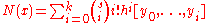
where no two xj are the same, the interpolation polynomial in the Newton form is a linear combination
of Newton basis polynomials
with the Newton basis polynomials defined as
for and
and  . The coefficients are defined as
where

is the notation for divided differences
.
Thus the Newton polynomial can be written as

The Newton Polynomial above can be expressed in a simplified form when are arranged consecutively with equal space. Introducing the notation
  for each
 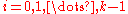 and
and  , the difference
  can be written as
  . So the Newton Polynomial above becomes:

is called the Newton Forward Divided Difference Formula.
If the nodes are reordered as , the Newton Polynomial becomes:

If are equally spaced with x=
 and
and 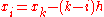 for
for  , then,


is called the Newton Backward Divided Difference Formula.
Gauss's formula alternately adds new points at the left and right ends, thereby keeping the set of points centered near the same place (near the evaluated point). When so doing, it uses terms from Newton's formula, with data points and x values re-named in keeping with one's choice of what data point is designated as the data point.
Stirling's formula remains centered about a particular data point, for use when the evaluated point is nearer to a data point than to a middle of two data points. Bessel's formula remains centered about a particular middle between two data points, for use when the evaluated point is nearer to a middle than to a data point. They achieve that by sometimes using the average of two differences where Newton's or Gauss's would use just one difference. Stirling's does that in odd-degree terms; Bessels does that in even-degree terms. Calculating and averaging two differences need not involve extra work, since it can be done by formula, in advance—the expression for the averaged difference is not more complicated than that of the simple difference.
In general, the difference methods can be a good choice when one does not know how many points, what degree of interpolating polynomial, will be needed for the desired accuracy, and when one wants to look first at linear and other low-degree interpolation, successively judging accuracy by the difference in the results of two successive polynomial degrees. Lagrange's formula (not a difference formula) allows that also, but going to the next higher degree without re-doing work requires that each term's value be recorded—not a problem with a computer, but maybe awkward with a calculator.
Other than that, Lagrange is easier to calculate than the difference methods, and is (probably rightly) regarded by many as the best choice when one already knows what polynomial degree will be needed. And when all the interpolation will be done at one x value, with only the data points' y values varying from one problem to another, Lagrange's formula becomes so much more convenient that it begins to be the only choice to consider.
Lagrange's formula's ease of calculation is best achieved by its "barycentric forms". Its 2nd barycentric form might be the most efficient of all when using a computer, but its 1st barycentric form might be more convenient when using a calculator.
 , then as the evaluated point approaches that data point, the difference formula terms after the constant term tend toward zero. Therefore, Stirling's formula is at its best in the region where it is less needed. Bessel's is at its best when the evaluated point is near the middle between two data points, and therefore Bessel's is at its best when the added accuracy is most needed. So, Bessel's formula could be said to be the most consistently accurate difference formula, and, in general, the most consistently accurate of the familiar polynomial interpolation formulas.
It should be added that, when Bessel's or Stirling's gains a little accuracy over Gauss's and Lagrange's, it would be unusual for that extra accuracy to be needed. No one should quit using Lagrange's or Gauss's because of it.
When, with Stirling's or Bessel's, the last term used includes the average of two differences, then one more point is being used than Newton's or other polynomial interpolations would use for the same polynomial degree. So, in that instance, Stirling's or Bessel's is not putting an N-1 degree polynomial through N points, but is, instead, trading equivalence with Newton's for better centering and accuracy, giving those methods sometimes potentially greater accuracy, for a given polynomial degree, than other polynomial interpolations.
The other difference formulas, such as those of Stirling, Bessel and Gauss, can be derived from Newton's, using Newton's terms, with data points and x values renamed in keeping with the choice of x zero, and based on the fact that they must add up to the same sum value as Newton's (With Stirling that is so when polynomial degree is even. With Bessel's that is so when polynomial degree is odd).
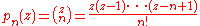
 , there is a closely related set of polynomials, also called the Newton polynomials, that are simply the binomial coefficient
s for general argument. That is, one also has the Newton polynomials given by
In this form, the Newton polynomials generate the Newton series. These are in turn a special case of the general difference polynomials which allow the representation of analytic function
s through generalized difference equations.
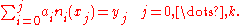
for our interpolation polynomial we get the very complicated Vandermonde matrix. By choosing another basis, the Newton basis, we get a system of linear equations with a much simpler lower triangular matrix which can be solved faster.
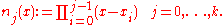
For k + 1 data points we construct the Newton basis as
Using these polynomials as a basis for we have to solve
to solve the polynomial interpolation problem.
This system of equations can be solved recursively by solving
because the divided differences become derivatives.
Numerical analysis
Numerical analysis is the study of algorithms that use numerical approximation for the problems of mathematical analysis ....
, a Newton polynomial, named after its inventor Isaac Newton
Isaac Newton
Sir Isaac Newton PRS was an English physicist, mathematician, astronomer, natural philosopher, alchemist, and theologian, who has been "considered by many to be the greatest and most influential scientist who ever lived."...
, is the interpolation
Polynomial interpolation
In numerical analysis, polynomial interpolation is the interpolation of a given data set by a polynomial: given some points, find a polynomial which goes exactly through these points.- Applications :...
polynomial
Polynomial
In mathematics, a polynomial is an expression of finite length constructed from variables and constants, using only the operations of addition, subtraction, multiplication, and non-negative integer exponents...
for a given set of data points in the Newton form. The Newton polynomial is sometimes called Newton's divided differences interpolation polynomial because the coefficients of the polynomial are calculated using divided differences
Divided differences
In mathematics divided differences is a recursive division process.The method can be used to calculate the coefficients in the interpolation polynomial in the Newton form.-Definition:Given n data points,\ldots,...
.
For any given set of data points, there is only one polynomial (of least possible degree) that passes through all of them. Thus, it is more appropriate to speak of "the Newton form of the interpolation polynomial" rather than of "the Newton interpolation polynomial". Like the Lagrange form
Lagrange polynomial
In numerical analysis, Lagrange polynomials are used for polynomial interpolation. For a given set of distinct points x_j and numbers y_j, the Lagrange polynomial is the polynomial of the least degree that at each point x_j assumes the corresponding value y_j...
, it is merely another way to write the same polynomial.
Definition
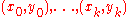
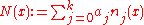
Given a set of k + 1 data pointswhere no two xj are the same, the interpolation polynomial in the Newton form is a linear combination
Linear combination
In mathematics, a linear combination is an expression constructed from a set of terms by multiplying each term by a constant and adding the results...
of Newton basis polynomials
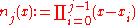
with the Newton basis polynomials defined as
for
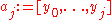
and . The coefficients are defined aswhere
is the notation for divided differences
Divided differences
In mathematics divided differences is a recursive division process.The method can be used to calculate the coefficients in the interpolation polynomial in the Newton form.-Definition:Given n data points,\ldots,...
.
Thus the Newton polynomial can be written as
The Newton Polynomial above can be expressed in a simplified form when
are arranged consecutively with equal space. Introducing the notation for each and , the difference can be written as . So the Newton Polynomial above becomes:is called the Newton Forward Divided Difference Formula.
If the nodes are reordered as
, the Newton Polynomial becomes:If
are equally spaced with x= and for , then,is called the Newton Backward Divided Difference Formula.
Significance
Newton's formula is of interest because it is the straightforward and natural differences-version of Taylor's polynomial. Taylor's polynomial tells where a function will go, based on its y value, and its derivatives (its rate of change, and the rate of change of its rate of change, etc.) at one particular x value. Newton's formula is Taylor's polynomial based on finite differences instead of instantaneous rates of change.Addition of new points
As with other difference formulas, the degree of a Newton's interpolating polynomial can be increased by adding more terms and points without discarding existing ones. Newton's form has the simplicity that the new points are always added at one end: Newton's forward formula can add new points to the right, and Newton's backwards formula can add new points to the left. Unfortunately, the accuracy of polynomial interpolation depends on how close the interpolated point is to the middle of the x values of the set of points used; as Newton's form always adds new points at the same end, an increase in degree cannot be used to increase the accuracy anywhere but at that end. Gauss, Stirling, and Bessel all developed formulae to remedy that problem.Gauss's formula alternately adds new points at the left and right ends, thereby keeping the set of points centered near the same place (near the evaluated point). When so doing, it uses terms from Newton's formula, with data points and x values re-named in keeping with one's choice of what data point is designated as the
data point.Stirling's formula remains centered about a particular data point, for use when the evaluated point is nearer to a data point than to a middle of two data points. Bessel's formula remains centered about a particular middle between two data points, for use when the evaluated point is nearer to a middle than to a data point. They achieve that by sometimes using the average of two differences where Newton's or Gauss's would use just one difference. Stirling's does that in odd-degree terms; Bessels does that in even-degree terms. Calculating and averaging two differences need not involve extra work, since it can be done by formula, in advance—the expression for the averaged difference is not more complicated than that of the simple difference.
Strengths and weaknesses of various formulae
The suitability of Stirling's, Bessel's and Gauss's formulae depends on 1) the importance of the small accuracy gain given by average differences; and 2) if greater accuracy is necessary, whether the interpolated point is closer to a data point or to a middle between two data points.In general, the difference methods can be a good choice when one does not know how many points, what degree of interpolating polynomial, will be needed for the desired accuracy, and when one wants to look first at linear and other low-degree interpolation, successively judging accuracy by the difference in the results of two successive polynomial degrees. Lagrange's formula (not a difference formula) allows that also, but going to the next higher degree without re-doing work requires that each term's value be recorded—not a problem with a computer, but maybe awkward with a calculator.
Other than that, Lagrange is easier to calculate than the difference methods, and is (probably rightly) regarded by many as the best choice when one already knows what polynomial degree will be needed. And when all the interpolation will be done at one x value, with only the data points' y values varying from one problem to another, Lagrange's formula becomes so much more convenient that it begins to be the only choice to consider.
Lagrange's formula's ease of calculation is best achieved by its "barycentric forms". Its 2nd barycentric form might be the most efficient of all when using a computer, but its 1st barycentric form might be more convenient when using a calculator.
Accuracy
When a particular data point is designated as, then as the evaluated point approaches that data point, the difference formula terms after the constant term tend toward zero. Therefore, Stirling's formula is at its best in the region where it is less needed. Bessel's is at its best when the evaluated point is near the middle between two data points, and therefore Bessel's is at its best when the added accuracy is most needed. So, Bessel's formula could be said to be the most consistently accurate difference formula, and, in general, the most consistently accurate of the familiar polynomial interpolation formulas.It should be added that, when Bessel's or Stirling's gains a little accuracy over Gauss's and Lagrange's, it would be unusual for that extra accuracy to be needed. No one should quit using Lagrange's or Gauss's because of it.
When, with Stirling's or Bessel's, the last term used includes the average of two differences, then one more point is being used than Newton's or other polynomial interpolations would use for the same polynomial degree. So, in that instance, Stirling's or Bessel's is not putting an N-1 degree polynomial through N points, but is, instead, trading equivalence with Newton's for better centering and accuracy, giving those methods sometimes potentially greater accuracy, for a given polynomial degree, than other polynomial interpolations.
The other difference formulas, such as those of Stirling, Bessel and Gauss, can be derived from Newton's, using Newton's terms, with data points and x values renamed in keeping with the choice of x zero, and based on the fact that they must add up to the same sum value as Newton's (With Stirling that is so when polynomial degree is even. With Bessel's that is so when polynomial degree is odd).
General case
For the special case of, there is a closely related set of polynomials, also called the Newton polynomials, that are simply the binomial coefficientBinomial coefficient
In mathematics, binomial coefficients are a family of positive integers that occur as coefficients in the binomial theorem. They are indexed by two nonnegative integers; the binomial coefficient indexed by n and k is usually written \tbinom nk , and it is the coefficient of the x k term in...
s for general argument. That is, one also has the Newton polynomials
given byIn this form, the Newton polynomials generate the Newton series. These are in turn a special case of the general difference polynomials which allow the representation of analytic function
Analytic function
In mathematics, an analytic function is a function that is locally given by a convergent power series. There exist both real analytic functions and complex analytic functions, categories that are similar in some ways, but different in others...
s through generalized difference equations.
Main idea
Solving an interpolation problem leads to a problem in linear algebra where we have to solve a system of linear equations. Using a standard monomial basisMonomial basis
In mathematics a monomial basis is a way to describe uniquely a polynomial using a linear combination of monomials. This description, the monomial form of a polynomial, is often used because of the simple structure of the monomial basis....
for our interpolation polynomial we get the very complicated Vandermonde matrix. By choosing another basis, the Newton basis, we get a system of linear equations with a much simpler lower triangular matrix which can be solved faster.
For k + 1 data points we construct the Newton basis as
Using these polynomials as a basis for
we have to solveto solve the polynomial interpolation problem.
This system of equations can be solved recursively by solving
Taylor polynomial
The limit of the Newton polynomial if all nodes coincide is a Taylor polynomial,because the divided differences become derivatives.
-

Application
As can be seen from the definition of the divided differences new data points can be added to the data set to create a new interpolation polynomial without recalculating the old coefficients. And when a data point changes we usually do not have to recalculate all coefficients. Furthermore if the xi are distributed equidistantly the calculation of the divided differences becomes significantly easier. Therefore the Newton form of the interpolation polynomial is usually preferred over the Lagrange formLagrange polynomialIn numerical analysis, Lagrange polynomials are used for polynomial interpolation. For a given set of distinct points x_j and numbers y_j, the Lagrange polynomial is the polynomial of the least degree that at each point x_j assumes the corresponding value y_j...
for practical purposes, although, in actual fact (and contrary to widespread claims), Lagrange, too, allows calculation of the next higher degree interpolation without re-doing previous calculations—and is considerably easier to evaluate.
Example
The divided differences can be written in the form of a table. For example, for a function is to be interpolated on points
  . Write
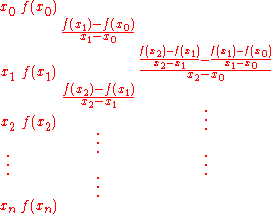
Then the interpolating polynomial is formed as above using the topmost entries in each column as coefficients.
For example, suppose we are to construct the interpolating polynomial to using divided differences, at the points


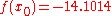


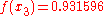
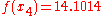
Using six digits of accuracy, we construct the table-
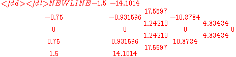
Thus, the interpolating polynomial is
Given more digits of accuracy in the table, the first and third coefficients will
be found to be zero.
See also
- Newton series
- Neville's schema
- Polynomial interpolationPolynomial interpolationIn numerical analysis, polynomial interpolation is the interpolation of a given data set by a polynomial: given some points, find a polynomial which goes exactly through these points.- Applications :...
- Lagrange formLagrange polynomialIn numerical analysis, Lagrange polynomials are used for polynomial interpolation. For a given set of distinct points x_j and numbers y_j, the Lagrange polynomial is the polynomial of the least degree that at each point x_j assumes the corresponding value y_j...
of the interpolation polynomial - Bernstein formBernstein polynomialIn the mathematical field of numerical analysis, a Bernstein polynomial, named after Sergei Natanovich Bernstein, is a polynomial in the Bernstein form, that is a linear combination of Bernstein basis polynomials....
of the interpolation polynomial - Hermite interpolationHermite interpolationIn numerical analysis, Hermite interpolation, named after Charles Hermite, is a method of interpolating data points as a polynomial function. The generated Hermite polynomial is closely related to the Newton polynomial, in that both are derived from the calculation of divided differences.Unlike...
External links
-
-

