

Multivariate kernel density estimation
Encyclopedia
Kernel density estimation
is a nonparametric technique for density estimation
i.e., estimation of probability density function
s, which is one of the fundamental questions in statistics
. It can be viewed as a generalisation of histogram
density estimation with improved statistical properties. Apart from histograms, other types of density estimators include parametric
, spline
, wavelet
and Fourier series
. Kernel density estimators were first introduced in the scientific literature for univariate
data in the 1950s and 1960s and subsequently have been widely adopted. It was soon recognised that analogous estimators for multivariate data would be an important addition to multivariate statistics
. Based on research carried out in the 1990s and 2000s, multivariate kernel density estimation has reached a level of maturity comparable to their univariate counterparts.
data set of 50 points to illustrate the construction of histograms. This requires the choice of an anchor point (the lower left corner of the histogram grid). For the histogram on the left, we choose (−1.5, −1.5): for the one on the right, we shift the anchor point by 0.125 in both directions to (−1.625, −1.625). Both histograms have a binwidth of 0.5, so any differences are due to the change in the anchor point only. The colour coding indicates the number of data points which fall into a bin: 0=white, 1=pale yellow, 2=bright yellow, 3=orange, 4=red. The left histogram appears to indicate that the upper half has a higher density than the lower half, whereas it is the reverse is the case for the right-hand histogram, confirming that histograms are highly sensitive to the placement of the anchor point.
One possible solution to this anchor point placement problem is to remove the histogram binning grid completely. In the left figure below, a kernel (represented by the grey lines) is centred at each of the 50 data points above. The result of summing these kernels is given on the right figure, which is a kernel density estimate. The most striking difference between kernel density estimates and histograms is that the former are easier to interpret since they do not contain artifices induced by a binning grid.
The coloured contours correspond to the smallest region which contains the respective probability mass: red = 25%, orange + red = 50%, yellow + orange + red = 75%, thus indicating that a single central region contains the highest density.
The goal of density estimation is to take a finite sample of data and to make inferences about the underyling probability density function everywhere, including where no data are observed. In kernel density estimation, the contribution of each data point is smoothed out from a single point into a region of space surrounding it. Aggregating the individually smoothed contributions gives an overall picture of the structure of the data and its density function. In the details to follow, we show that this approach leads to a reasonable estimate of the underlying density function.
of d-variate random vectors drawn from a common distribution described by the density function
ƒ. The kernel density estimate is defined to be
Kernel density estimation
In statistics, kernel density estimation is a non-parametric way of estimating the probability density function of a random variable. Kernel density estimation is a fundamental data smoothing problem where inferences about the population are made, based on a finite data sample...
is a nonparametric technique for density estimation
Density estimation
In probability and statistics,density estimation is the construction of an estimate, based on observed data, of an unobservable underlying probability density function...
i.e., estimation of probability density function
Probability density function
In probability theory, a probability density function , or density of a continuous random variable is a function that describes the relative likelihood for this random variable to occur at a given point. The probability for the random variable to fall within a particular region is given by the...
s, which is one of the fundamental questions in statistics
Statistics
Statistics is the study of the collection, organization, analysis, and interpretation of data. It deals with all aspects of this, including the planning of data collection in terms of the design of surveys and experiments....
. It can be viewed as a generalisation of histogram
Histogram
In statistics, a histogram is a graphical representation showing a visual impression of the distribution of data. It is an estimate of the probability distribution of a continuous variable and was first introduced by Karl Pearson...
density estimation with improved statistical properties. Apart from histograms, other types of density estimators include parametric
Parametric statistics
Parametric statistics is a branch of statistics that assumes that the data has come from a type of probability distribution and makes inferences about the parameters of the distribution. Most well-known elementary statistical methods are parametric....
, spline
Spline interpolation
In the mathematical field of numerical analysis, spline interpolation is a form of interpolation where the interpolant is a special type of piecewise polynomial called a spline. Spline interpolation is preferred over polynomial interpolation because the interpolation error can be made small even...
, wavelet
Wavelet
A wavelet is a wave-like oscillation with an amplitude that starts out at zero, increases, and then decreases back to zero. It can typically be visualized as a "brief oscillation" like one might see recorded by a seismograph or heart monitor. Generally, wavelets are purposefully crafted to have...
and Fourier series
Fourier series
In mathematics, a Fourier series decomposes periodic functions or periodic signals into the sum of a set of simple oscillating functions, namely sines and cosines...
. Kernel density estimators were first introduced in the scientific literature for univariate
Univariate
In mathematics, univariate refers to an expression, equation, function or polynomial of only one variable. Objects of any of these types but involving more than one variable may be called multivariate...
data in the 1950s and 1960s and subsequently have been widely adopted. It was soon recognised that analogous estimators for multivariate data would be an important addition to multivariate statistics
Multivariate statistics
Multivariate statistics is a form of statistics encompassing the simultaneous observation and analysis of more than one statistical variable. The application of multivariate statistics is multivariate analysis...
. Based on research carried out in the 1990s and 2000s, multivariate kernel density estimation has reached a level of maturity comparable to their univariate counterparts.
Motivation
We take an illustrative synthetic bivariateBivariate data
In mathematics, bivariate data is data that involves two variables. The quantities from these two variables are often represented using a scatter plot...
data set of 50 points to illustrate the construction of histograms. This requires the choice of an anchor point (the lower left corner of the histogram grid). For the histogram on the left, we choose (−1.5, −1.5): for the one on the right, we shift the anchor point by 0.125 in both directions to (−1.625, −1.625). Both histograms have a binwidth of 0.5, so any differences are due to the change in the anchor point only. The colour coding indicates the number of data points which fall into a bin: 0=white, 1=pale yellow, 2=bright yellow, 3=orange, 4=red. The left histogram appears to indicate that the upper half has a higher density than the lower half, whereas it is the reverse is the case for the right-hand histogram, confirming that histograms are highly sensitive to the placement of the anchor point.
One possible solution to this anchor point placement problem is to remove the histogram binning grid completely. In the left figure below, a kernel (represented by the grey lines) is centred at each of the 50 data points above. The result of summing these kernels is given on the right figure, which is a kernel density estimate. The most striking difference between kernel density estimates and histograms is that the former are easier to interpret since they do not contain artifices induced by a binning grid.
The coloured contours correspond to the smallest region which contains the respective probability mass: red = 25%, orange + red = 50%, yellow + orange + red = 75%, thus indicating that a single central region contains the highest density.
The goal of density estimation is to take a finite sample of data and to make inferences about the underyling probability density function everywhere, including where no data are observed. In kernel density estimation, the contribution of each data point is smoothed out from a single point into a region of space surrounding it. Aggregating the individually smoothed contributions gives an overall picture of the structure of the data and its density function. In the details to follow, we show that this approach leads to a reasonable estimate of the underlying density function.
Definition
The previous figure is a graphical representation of kernel density estimate, which we now define in an exact manner. Let x1, x2, …, xn be a sampleRandom sample
In statistics, a sample is a subject chosen from a population for investigation; a random sample is one chosen by a method involving an unpredictable component...
of d-variate random vectors drawn from a common distribution described by the density function
Probability density function
In probability theory, a probability density function , or density of a continuous random variable is a function that describes the relative likelihood for this random variable to occur at a given point. The probability for the random variable to fall within a particular region is given by the...
ƒ. The kernel density estimate is defined to be
-

where (x1, x2, …, xd)T}}, are d-vectors;- H is the bandwidth (or smoothing) d×d matrix which is symmetric and positive definite;
- K is the kernelKernel (statistics)A kernel is a weighting function used in non-parametric estimation techniques. Kernels are used in kernel density estimation to estimate random variables' density functions, or in kernel regression to estimate the conditional expectation of a random variable. Kernels are also used in time-series,...
function which is a symmetric multivariate density; H−1/2 K(H−1/2x)}}.
The choice of the kernel function K is not crucial to the accuracy of kernel density estimators, so we use the standard multivariate normal kernel throughout: . Whereas the choice of the bandwidth matrix H is the single most important factor affecting its accuracy since it controls the amount of and orientation of smoothing induced. That the bandwidth matrix also induces an orientation is a basic difference between multivariate kernel density estimation from its univariate analogue since orientation is not defined for 1D kernels. This leads to the choice of the parametrisation of this bandwidth matrix. The three main parametrisation classes (in increasing order of complexity) are S, the class of positive scalars times the identity matrix; D, diagonal matrices with positive entries on the main diagonal; and F, symmetric positive definite matrices. The S class kernels have the same amount of smoothing applied in all coordinate directions, D kernels allow different amounts of smoothing in each of the coordinates, and F kernels allow arbitrary amounts and orientation of the smoothing. Historically S and D kernels are the most widespread due to computational reasons, but research indicates that important gains in accuracy can be obtained using the more general F class kernels.
Optimal bandwidth matrix selection
The most commonly used optimality criterion for selecting a bandwidth matrix is the MISE or mean integrated squared error
This in general does not possess a closed-form expressionClosed-form expressionIn mathematics, an expression is said to be a closed-form expression if it can be expressed analytically in terms of a bounded number of certain "well-known" functions...
, so it is usual to use its asymptotic approximation (AMISE) as a proxy
-

where
 , with when K is a normal kernel
 ,
,
with Id being the d × d identity matrixIdentity matrixIn linear algebra, the identity matrix or unit matrix of size n is the n×n square matrix with ones on the main diagonal and zeros elsewhere. It is denoted by In, or simply by I if the size is immaterial or can be trivially determined by the context...
, with m2 = 1 for the normal kernel
- D2ƒ is the d × d Hessian matrix of second order partial derivatives of ƒ
 is a d2 × d2 matrix of integrated fourth order
partial derivatives of ƒ
- vec is the vector operator which stacks the columns of a matrix into a single vector e.g.
The quality of the AMISE approximation to the MISE is given by
where o indicates the usual small o notationBig O notationIn mathematics, big O notation is used to describe the limiting behavior of a function when the argument tends towards a particular value or infinity, usually in terms of simpler functions. It is a member of a larger family of notations that is called Landau notation, Bachmann-Landau notation, or...
. Heuristically this statement implies that the AMISE is a 'good' approximation of the MISE as the sample size n → ∞.
It can be shown that any reasonable bandwidth selector H has H = O(n-2/(d+4)) where the big O notationBig O notationIn mathematics, big O notation is used to describe the limiting behavior of a function when the argument tends towards a particular value or infinity, usually in terms of simpler functions. It is a member of a larger family of notations that is called Landau notation, Bachmann-Landau notation, or...
is applied elementwise. Substituting this into the MISE formula yields that the optimal MISE is O(n-4/(d+4)). Thus as n → ∞, the MISE → 0, i.e. the kernel density estimate converges in mean square and thus also in probability to the true density f. These modes of convergence are confirmation of the statement in the motivation section that kernel methods lead to reasonable density estimators. An ideal optimal bandwidth selector is
Since this ideal selector contains the unknown density function ƒ, it cannot be used directly. The many different varieties of data-based bandwidth selectors arise from the different estimators of the AMISE. We concentrate on two classes of selectors which have been shown to be the most widely applicable in practise: smoothed cross validation and plug-in selectors.
Plug-in
The plug-in (PI) estimate of the AMISE is formed by replacing Ψ4 by its estimator
-

where . Thus
  is the plug-in selector. These references also contain algorithms on optimal estimation of the pilot bandwidth matrix G and establish that
  converges in probability to HAMISE.
Smoothed cross validation
Smoothed cross validation (SCV) is a subset of a larger class of cross validation techniques. The SCV estimator differs from the plug-in estimator in the second term
-

Thus is the SCV selector.
These references also contain algorithms on optimal estimation of the pilot bandwidth matrix G and establish that converges in probability to HAMISE.
Asymptotic analysis
In the optimal bandwidth selection section, we introduced the MISE. Its construction relies on the expected valueExpected valueIn probability theory, the expected value of a random variable is the weighted average of all possible values that this random variable can take on...
and the varianceVarianceIn probability theory and statistics, the variance is a measure of how far a set of numbers is spread out. It is one of several descriptors of a probability distribution, describing how far the numbers lie from the mean . In particular, the variance is one of the moments of a distribution...
of the density esimator

where * is the convolutionConvolutionIn mathematics and, in particular, functional analysis, convolution is a mathematical operation on two functions f and g, producing a third function that is typically viewed as a modified version of one of the original functions. Convolution is similar to cross-correlation...
operator between two functions, and

For these two expressions to be well-defined, we require that all elements of H tend to 0 and that n-1 |H|-1/2 tends to 0 as n tends to infinity. Assuming these two conditions, we see that the expected value tends to the true density f i.e. the kernel density estimator is asymptotically unbiasedBias of an estimatorIn statistics, bias of an estimator is the difference between this estimator's expected value and the true value of the parameter being estimated. An estimator or decision rule with zero bias is called unbiased. Otherwise the estimator is said to be biased.In ordinary English, the term bias is...
; and that the variance tends to zero. Using the standard mean squared value decomposition

we have that the MSE tends to 0, implying that the kernel density estimator is (mean square) consistent and hence converges in probability to the true density f. The rate of convergence of the MSE to 0 is the necessarily the same as the MISE rate noted previously O(n-4/(d+4)), hence the covergence rate of the density estimator to f is Op(n-2/(d+4)) where Op denotes order in probabilityBig O in probability notationThe order in probability notation is used in probability theory and statistical theory in direct parallel to the big-O notation which is standard in mathematics...
. This establishes pointwise convergence. The functional covergence is established similarly by considering the behaviour of the MISE, and noting that under sufficient regularity, integration does not affect the convergence rates.
For the data-based bandwidth selectors considered, the target is the AMISE bandwidth matrix. We say that a data-based selector converges to the AMISE selector at relative rate Op(n-α), α > 0 if

It has been established that the plug-in and smoothed cross validation selectors (given a single pilot bandwidth G) both converge at a relative rate of Op(n-2/(d+6)) i.e., both these data-based selectors are consistent estimators.
Density estimation in R with a full bandwidth matrix
The ks package in R implements the plug-in and smoothed cross validation selectors (amongst others). This dataset (included in the base distribution of R) contains
272 records with two measurements each: the duration time of an eruprion (minutes) and the
waiting time until the next eruption (minutes) of the Old Faithful GeyserOld Faithful GeyserOld Faithful is a cone geyser located in Wyoming, in Yellowstone National Park in the United States. Old Faithful was named in 1870 during the Washburn-Langford-Doane Expedition and was the first geyser in the park to receive a name...
in Yellowstone National Park, USA.
The code fragment computes the kernel density estimate with the plug-in bandwidth matrix Again, the coloured contours correspond to the smallest region which contains the respective probability mass: red = 25%, orange + red = 50%, yellow + orange + red = 75%. To compute the SCV selector,
 Hpiis replaced withHscv. This is not displayed here since it is mostly similar to the plug-in estimate for this example.
library(ks)

data(faithful)

H <- Hpi(x=faithful)

fhat <- kde(x=faithful, H=H)

plot(fhat, display="filled.contour2")

points(faithful, cex=0.5, pch=16)
Density estimation in R with a diagonal bandwidth matrix
This example is again based on the Old Faithful Geyser, but this time we use the R np package that employs automatic (data-driven) bandwidth selection for a diagonal bandwidth matrix; see the np vignette for an introduction to the np package. The figure below shows the joint density estimate using a second order Gaussian kernel.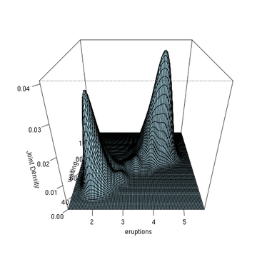
R script for the example
The following commands of the R programming language use the
npudens function to deliver optimal smoothing and to create
the figure given above. These commands can be entered at the command
prompt by using cut and paste.
 library(np)

 library(datasets)

 data(faithful)

 f <- npudens(~eruptions+waiting,data=faithful)

 plot(f,view="fixed",neval=100,phi=30,main="",xtrim=-0.2)
Density estimation in Matlab with a diagonal bandwidth matrix
We consider estimating the density of the Gaussian mixture
,
from 500 randomly generated points. We employ the Matlab routine for
2-dimensional data.
The routine is an automatic bandwidth selection method specifically designed
for a second order Gaussian kernel .
The figure shows the joint density estimate that results from using the automatically selected bandwidth.
Matlab script for the example
Type the following commands in Matlab after
downloading
and saving the function kde2d.m
in the current directory.
 clear all

 % generate synthetic data

data=[randn(500,2);

      randn(500,1)+3.5, randn(500,1);];

  % call the routine, which has been saved in the current directory

    [bandwidth,density,X,Y]=kde2d(data);

  % plot the data and the density estimate

    contour3(X,Y,density,50), hold on

    plot(data(:,1),data(:,2),'r.','MarkerSize',5)
Alternative optimality criteria
The MISE is the expected integrated L2 distance between the density estimate and the true density function f. It is the most widely used, mostly due to its tractability and most software implement MISE-based bandwidth selectors.
There are alternative optimality criteria, which attempt to cover cases where MISE is not an appropriate measure. The equivalent L1 measure, Mean Integrated Absolute Error, is
Its mathematical analysis is considerably more difficult than the MISE ones. In practise, the gain appears not to be significant. The L∞ norm is the Mean Uniform Absolute Error
which has been investigated only briefly. Likelihood error criteria include those based on the Mean Kullback-Leibler distance
and the Mean Hellinger distanceHellinger distanceIn probability and statistics, the Hellinger distance is used to quantify the similarity between two probability distributions. It is a type of f-divergence...
The KL can be estimated using a cross-validation method, although KL cross-validation selectors can be sub-optimal even if it remains consistentConsistent estimatorIn statistics, a sequence of estimators for parameter θ0 is said to be consistent if this sequence converges in probability to θ0...
for bounded density functions. MH selectors have been briefly examined in the literature.
All these optimality criteria are distance based measures, and do not always correspond to more intuitive notions of closeness, so more visual criteria have been developed in response to this concern.
External links
- www.mvstat.net/tduong/research A collection of peer-reviewed articles of the mathematical details of multivariate kernel density estimation and their bandwidth selectors.
- libagf A C++C++C++ is a statically typed, free-form, multi-paradigm, compiled, general-purpose programming language. It is regarded as an intermediate-level language, as it comprises a combination of both high-level and low-level language features. It was developed by Bjarne Stroustrup starting in 1979 at Bell...
library for multivariate, variable bandwidth kernel density estimation.
See also
- Kernel density estimationKernel density estimationIn statistics, kernel density estimation is a non-parametric way of estimating the probability density function of a random variable. Kernel density estimation is a fundamental data smoothing problem where inferences about the population are made, based on a finite data sample...
– univariate kernel density estimation. - Variable kernel density estimationVariable kernel density estimationIn statistics, adaptive or "variable-bandwidth" kernel density estimation is a form of kernel density estimation in which the size of the kernels used in the estimate are varied...
– estimation of multivariate densities using the kernel with variable bandwidth
-
-


