
Density estimation
Encyclopedia
In probability
and statistics
,
density estimation is the construction of an estimate, based on observed data
, of an unobservable underlying probability density function
. The unobservable density function is thought of as the density according to which a large population is distributed; the data are usually thought of as a random sample from that population.
A variety of approaches to density estimation are used, including Parzen windows and a range of data clustering
techniques, including vector quantization
. The most basic form of density estimation is a rescaled histogram
.
The following is quoted verbatim from the data set
description:
In this example,
we construct three density estimates for "glu" (plasma
glucose
concentration),
one conditional
on the presence of diabetes,
the second conditional on the absence of diabetes,
and the third not conditional on diabetes.
The conditional density estimates are then used to construct the probability of diabetes conditional on "glu".
The "glu" data were obtained from the MASS package of the R programming language. Within 'R', ?Pima.tr and ?Pima.te give a fuller account of the data.
The mean
of "glu" in the diabetes cases is 143.1 and the standard deviation is 31.26.
The mean of "glu" in the non-diabetes cases is 110.0 and the standard deviation is 24.29.
From this we see that, in this data set, diabetes cases are associated with greater levels of "glu".
This will be made clearer by plots of the estimated density functions.
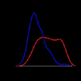
The first figure shows density estimates of p(glu | diabetes=1), p(glu | diabetes=0), and p(glu).
The density estimates are kernel density estimates using a Gaussian kernel.
That is,
a Gaussian density function is placed at each data point,
and the sum of the density functions is computed over the range of the data.
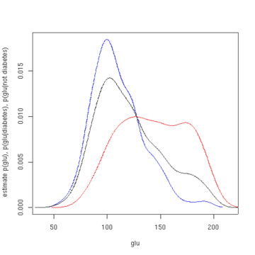
Estimated density of p(glu | diabetes=1) (red), p(glu | diabetes=0) (blue), and p(glu) (black).
From the density of "glu" conditional on diabetes,
we can obtain the probability of diabetes conditional on "glu" via Bayes' rule
.
For brevity, "diabetes" is abbreviated "db." in this formula.

The second figure shows the estimated posterior probability p(diabetes=1 | glu).
From these data,
it appears that an increased level of "glu" is associated with diabetes.
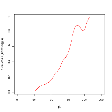
Estimated probability of p(diabetes=1 | glu).
These commands can be entered at the command prompt by using cut and paste.
library (MASS)
data(Pima.tr)
data(Pima.te)
Pima <- rbind (Pima.tr, Pima.te)
glu <- Pima[,'glu']
d0 <- Pima[,'type'] 'No'
'Yes'
base.rate.d1 <- sum(d1)/(sum(d1) + sum(d0))
glu.density <- density (glu)
glu.d0.density <- density (glu[d0])
glu.d1.density <- density (glu[d1])
approxfun (glu.d0.density$x, glu.d0.density$y) -> glu.d0.f
approxfun (glu.d1.density$x, glu.d1.density$y) -> glu.d1.f
p.d.given.glu <- function (glu, base.rate.d1)
{
p1 <- glu.d1.f(glu) * base.rate.d1
p0 <- glu.d0.f(glu) * (1 - base.rate.d1)
p1/(p0+p1)
}
x <- 1:250
y <- p.d.given.glu (x, base.rate.d1)
plot (x, y, type='l', col='red', xlab='glu', ylab='estimated p(diabetes|glu)')
plot (density(glu[d0]), col='blue', xlab='glu', ylab='estimate p(glu),
p(glu|diabetes), p(glu|not diabetes)', main=NA)
lines (density(glu[d1]), col='red')
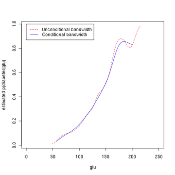
Note that the above conditional density estimator uses bandwidths
that are optimal for unconditional densities. Alternatively, one
could use the method of Hall, Racine and Li (2004) and the R np package
for automatic (data-driven) bandwidth selection that is
optimal for conditional density estimates; see the np vignette for an introduction to the np package. The following commands of the R programming language use the npcdens function to deliver optimal smoothing. Note that the response "Yes"/"No" is a factor.
library(np)
fy.x <- npcdens(type~glu,nmulti=1,data=Pima)
Pima.eval <- data.frame(type=factor("Yes"),
glu=seq(min(Pima$glu),max(Pima$glu),length=250))
plot (x, y, type='l', lty=2, col='red', xlab='glu',
ylab='estimated p(diabetes|glu)')
lines(Pima.eval$glu,predict(fy.x,newdata=Pima.eval),col="blue")
legend(0,1,c("Unconditional bandwidth", "Conditional bandwidth"),
col=c("red","blue"),lty=c(2,1))
The third figure uses optimal smoothing via the method of Hall, Racine, and Li (2004) indicating that the unconditional density bandwidth used in the second figure above yields a conditional density estimate that may be somewhat undersmoothed.
Estimated probability of p(diabetes=1 | glu).
Probability
Probability is ordinarily used to describe an attitude of mind towards some proposition of whose truth we arenot certain. The proposition of interest is usually of the form "Will a specific event occur?" The attitude of mind is of the form "How certain are we that the event will occur?" The...
and statistics
Statistics
Statistics is the study of the collection, organization, analysis, and interpretation of data. It deals with all aspects of this, including the planning of data collection in terms of the design of surveys and experiments....
,
density estimation is the construction of an estimate, based on observed data
Data
The term data refers to qualitative or quantitative attributes of a variable or set of variables. Data are typically the results of measurements and can be the basis of graphs, images, or observations of a set of variables. Data are often viewed as the lowest level of abstraction from which...
, of an unobservable underlying probability density function
Probability density function
In probability theory, a probability density function , or density of a continuous random variable is a function that describes the relative likelihood for this random variable to occur at a given point. The probability for the random variable to fall within a particular region is given by the...
. The unobservable density function is thought of as the density according to which a large population is distributed; the data are usually thought of as a random sample from that population.
A variety of approaches to density estimation are used, including Parzen windows and a range of data clustering
Data clustering
Cluster analysis or clustering is the task of assigning a set of objects into groups so that the objects in the same cluster are more similar to each other than to those in other clusters....
techniques, including vector quantization
Vector quantization
Vector quantization is a classical quantization technique from signal processing which allows the modeling of probability density functions by the distribution of prototype vectors. It was originally used for data compression. It works by dividing a large set of points into groups having...
. The most basic form of density estimation is a rescaled histogram
Histogram
In statistics, a histogram is a graphical representation showing a visual impression of the distribution of data. It is an estimate of the probability distribution of a continuous variable and was first introduced by Karl Pearson...
.
Example of density estimation
We will consider records of the incidence of diabetes.The following is quoted verbatim from the data set
Data set
A data set is a collection of data, usually presented in tabular form. Each column represents a particular variable. Each row corresponds to a given member of the data set in question. Its values for each of the variables, such as height and weight of an object or values of random numbers. Each...
description:
- A population of women who were at least 21 years old, of PimaPimaThe Pima are a group of American Indians living in an area consisting of what is now central and southern Arizona. The long name, "Akimel O'odham", means "river people". They are closely related to the Tohono O'odham and the Hia C-ed O'odham...
Indian heritage and living near Phoenix, Arizona, was tested for diabetes according to World Health OrganizationWorld Health OrganizationThe World Health Organization is a specialized agency of the United Nations that acts as a coordinating authority on international public health. Established on 7 April 1948, with headquarters in Geneva, Switzerland, the agency inherited the mandate and resources of its predecessor, the Health...
criteria. The data were collected by the US National Institute of Diabetes and Digestive and Kidney Diseases. We used the 532 complete records.
In this example,
we construct three density estimates for "glu" (plasma
Blood plasma
Blood plasma is the straw-colored liquid component of blood in which the blood cells in whole blood are normally suspended. It makes up about 55% of the total blood volume. It is the intravascular fluid part of extracellular fluid...
glucose
Glucose
Glucose is a simple sugar and an important carbohydrate in biology. Cells use it as the primary source of energy and a metabolic intermediate...
concentration),
one conditional
Conditional probability
In probability theory, the "conditional probability of A given B" is the probability of A if B is known to occur. It is commonly notated P, and sometimes P_B. P can be visualised as the probability of event A when the sample space is restricted to event B...
on the presence of diabetes,
the second conditional on the absence of diabetes,
and the third not conditional on diabetes.
The conditional density estimates are then used to construct the probability of diabetes conditional on "glu".
The "glu" data were obtained from the MASS package of the R programming language. Within 'R', ?Pima.tr and ?Pima.te give a fuller account of the data.
The mean
Mean
In statistics, mean has two related meanings:* the arithmetic mean .* the expected value of a random variable, which is also called the population mean....
of "glu" in the diabetes cases is 143.1 and the standard deviation is 31.26.
The mean of "glu" in the non-diabetes cases is 110.0 and the standard deviation is 24.29.
From this we see that, in this data set, diabetes cases are associated with greater levels of "glu".
This will be made clearer by plots of the estimated density functions.
The first figure shows density estimates of p(glu | diabetes=1), p(glu | diabetes=0), and p(glu).
The density estimates are kernel density estimates using a Gaussian kernel.
That is,
a Gaussian density function is placed at each data point,
and the sum of the density functions is computed over the range of the data.
From the density of "glu" conditional on diabetes,
we can obtain the probability of diabetes conditional on "glu" via Bayes' rule
Bayes' rule
In probability theory and applications, Bayes' rule relates the odds of event A_1 to event A_2, before and after conditioning on event B. The relationship is expressed in terms of the Bayes factor, \Lambda. Bayes' rule is derived from and closely related to Bayes' theorem...
.
For brevity, "diabetes" is abbreviated "db." in this formula.
The second figure shows the estimated posterior probability p(diabetes=1 | glu).
From these data,
it appears that an increased level of "glu" is associated with diabetes.
Script for example
The following commands of the R programming language will create the figures shown above.These commands can be entered at the command prompt by using cut and paste.
library (MASS)
data(Pima.tr)
data(Pima.te)
Pima <- rbind (Pima.tr, Pima.te)
glu <- Pima[,'glu']
d0 <- Pima[,'type']
'No'
d1 <- Pima[,'type']
'Yes'base.rate.d1 <- sum(d1)/(sum(d1) + sum(d0))
glu.density <- density (glu)
glu.d0.density <- density (glu[d0])
glu.d1.density <- density (glu[d1])
approxfun (glu.d0.density$x, glu.d0.density$y) -> glu.d0.f
approxfun (glu.d1.density$x, glu.d1.density$y) -> glu.d1.f
p.d.given.glu <- function (glu, base.rate.d1)
{
p1 <- glu.d1.f(glu) * base.rate.d1
p0 <- glu.d0.f(glu) * (1 - base.rate.d1)
p1/(p0+p1)
}
x <- 1:250
y <- p.d.given.glu (x, base.rate.d1)
plot (x, y, type='l', col='red', xlab='glu', ylab='estimated p(diabetes|glu)')
plot (density(glu[d0]), col='blue', xlab='glu', ylab='estimate p(glu),
p(glu|diabetes), p(glu|not diabetes)', main=NA)
lines (density(glu[d1]), col='red')
Note that the above conditional density estimator uses bandwidths
that are optimal for unconditional densities. Alternatively, one
could use the method of Hall, Racine and Li (2004) and the R np package
for automatic (data-driven) bandwidth selection that is
optimal for conditional density estimates; see the np vignette for an introduction to the np package. The following commands of the R programming language use the npcdens function to deliver optimal smoothing. Note that the response "Yes"/"No" is a factor.
library(np)
fy.x <- npcdens(type~glu,nmulti=1,data=Pima)
Pima.eval <- data.frame(type=factor("Yes"),
glu=seq(min(Pima$glu),max(Pima$glu),length=250))
plot (x, y, type='l', lty=2, col='red', xlab='glu',
ylab='estimated p(diabetes|glu)')
lines(Pima.eval$glu,predict(fy.x,newdata=Pima.eval),col="blue")
legend(0,1,c("Unconditional bandwidth", "Conditional bandwidth"),
col=c("red","blue"),lty=c(2,1))
The third figure uses optimal smoothing via the method of Hall, Racine, and Li (2004) indicating that the unconditional density bandwidth used in the second figure above yields a conditional density estimate that may be somewhat undersmoothed.
See also
- Kernel density estimationKernel density estimationIn statistics, kernel density estimation is a non-parametric way of estimating the probability density function of a random variable. Kernel density estimation is a fundamental data smoothing problem where inferences about the population are made, based on a finite data sample...
- Mean integrated squared error
- HistogramHistogramIn statistics, a histogram is a graphical representation showing a visual impression of the distribution of data. It is an estimate of the probability distribution of a continuous variable and was first introduced by Karl Pearson...
- Multivariate kernel density estimationMultivariate kernel density estimationKernel density estimation is a nonparametric technique for density estimation i.e., estimation of probability density functions, which is one of the fundamental questions in statistics. It can be viewed as a generalisation of histogram density estimation with improved statistical properties...
External links
- CREEM: Centre for Research Into Ecological and Environmental Modelling Downloads for free density estimation software packages Distance 4 (from Research Unit for Wildlife Population Assessment "RUWPA") and WiSP.
- UCI Machine Learning Repository Content Summary (See "Pima Indians Diabetes Database" for the original data set of 732 records, and additional notes.)
- Free MATLAB code for one and two dimensional density estimation
- The np package An RR (programming language)R is a programming language and software environment for statistical computing and graphics. The R language is widely used among statisticians for developing statistical software, and R is widely used for statistical software development and data analysis....
package that provides a variety of nonparametric and semiparametric kernel methods that seamlessly handle a mix of continuous, unordered, and ordered factor data types. - libAGF C++ software for variable kernel density estimationVariable kernel density estimationIn statistics, adaptive or "variable-bandwidth" kernel density estimation is a form of kernel density estimation in which the size of the kernels used in the estimate are varied...
.