
.gif)
State space (controls)
Encyclopedia
In control engineering
, a state space representation is a mathematical model of a physical system as a set of input, output and state variables related by first-order differential equation
s. To abstract from the number of inputs, outputs and states, the variables are expressed as vectors, and the differential and algebraic equations are written in matrix form (the last one can be done when the dynamical system
is linear and time invariant). The state space representation (also known as the "time-domain approach") provides a convenient and compact way to model and analyze systems with multiple inputs and outputs. With inputs and
  outputs, we would otherwise have to write down
  Laplace transforms to encode all the information about a system. Unlike the frequency domain approach, the use of the state space representation is not limited to systems with linear components and zero initial conditions. "State space" refers to the space whose axes are the state variables. The state of the system can be represented as a vector within that space.
 The internal state variable
s are the smallest possible subset of system variables that can represent the entire state of the system at any given time. The minimum number of state variables required to represent a given system, , is usually equal to the order of the system's defining differential equation. If the system is represented in transfer function form, the minimum number of state variables is equal to the order of the transfer function's denominator after it has been reduced to a proper fraction. It is important to understand that converting a state space realization to a transfer function form may lose some internal information about the system, and may provide a description of a system which is stable, when the state-space realization is unstable at certain points. In electric circuits, the number of state variables is often, though not always, the same as the number of energy storage elements in the circuit such as capacitor
s and inductor
s. The state variables defined must be linearly independent; no state variable can be written as a linear combination of the other state variables or the system will not be able to be solved.
 inputs,
  outputs and
  state variables is written in the following form:
where: is called the "state vector",
  ;
; is called the "output vector",
  ;
; is called the "input (or control) vector",
  ;
; is the "state matrix",
  ,
, is the "input matrix",
  ,
, is the "output matrix",
  ,
, is the "feedthrough (or feedforward) matrix" (in cases where the system model does not have a direct feedthrough,
  is the zero matrix),
  ,
,
In this general formulation, all matrices are allowed to be time-variant (i.e., their elements can depend on time); however, in the common LTI case, matrices will be time invariant. The time variable can be a "continuous" (e.g.,
  ) or discrete (e.g.,
  ). In the latter case, the time variable is usually indicated as
  . Hybrid system
s allow for time domains that have both continuous and discrete parts. Depending on the assumptions taken, the state-space model representation can assume the following forms:
in factored form. It will then look something like this:
The denominator of the transfer function is equal to the characteristic polynomial
found by taking the determinant
of ,
,
The roots of this polynomial (the eigenvalues) are the system transfer function's poles (i.e., the singularities
where the transfer function's magnitude is unbounded). These poles can be used to analyze whether the system is asymptotically stable or marginally stable
. An alternative approach to determining stability, which does not involve calculating eigenvalues, is to analyze the system's Lyapunov stability
.
The zeros found in the numerator of can similarly be used to determine whether the system is minimum phase
.
The system may still be input–output stable (see BIBO stable
) even though it is not internally stable. This may be the case if unstable poles are canceled out by zeros (i.e., if those singularities in the transfer function are removable).

Where rank
is the number of linearly independent rows in a matrix.
A continuous time-invariant linear state-space model is observable if and only if
" of a continuous time-invariant linear state-space model can be derived in the following way:
First, taking the Laplace transform of
yields
Next, we simplify for , giving
and thus
Substituting for in the output equation
 giving
Because the transfer function
 is defined as the ratio of the output to the input of a system, we take
and substitute the previous expression for with respect to
  , giving
Clearly must have
  by
by  dimensionality, and thus has a total of
  elements.
So for every input there are transfer functions with one for each output.
This is why the state-space representation can easily be the preferred choice for multiple-input, multiple-output (MIMO) systems.
can easily be transferred into state-space by the following approach (this example is for a 4-dimensional, single-input, single-output system)):
Given a transfer function, expand it to reveal all coefficients in both the numerator and denominator. This should result in the following form:
The coefficients can now be inserted directly into the state-space model by the following approach:

This state-space realization is called controllable canonical form because the resulting model is guaranteed to be controllable (i.e., because the control enters a chain of integrators, it has the ability to move every state).
The transfer function coefficients can also be used to construct another type of canonical form

This state-space realization is called observable canonical form because the resulting model is guaranteed to be observable (i.e., because the output exists from a chain of integrators, every state has an effect on the output).
(and not strictly proper
) can also be realised quite easily. The trick here is to separate the transfer function into two parts: a strictly proper part and a constant.
The strictly proper transfer function can then be transformed into a canonical state space realization using techniques shown above. The state space realization of the constant is trivially . Together we then get a state space realization with matrices A,B and C determined by the strictly proper part, and matrix D determined by the constant.
Here is an example to clear things up a bit:
which yields the following controllable realization

Notice how the output also depends directly on the input. This is due to the constant in the transfer function.
 A common method for feedback is to multiply the output by a matrix K and setting this as the input to the system:
  .
.
Since the values of K are unrestricted the values can easily be negated for negative feedback
.
The presence of a negative sign (the common notation) is merely a notational one and its absence has no impact on the end results.
becomes
solving the output equation for and substituting in the state equation results in
The advantage of this is that the eigenvalues of A can be controlled by setting K appropriately through eigendecomposition of .
.
This assumes that the closed-loop system is controllable
or that the unstable eigenvalues of A can be made stable through appropriate choice of K.
. This would then result in the simpler equations
This reduces the necessary eigendecomposition to just .
.
 In addition to feedback, an input,
  , can be added such that
  .
.
becomes
solving the output equation for and substituting in the state equation
results in
One fairly common simplification to this system is removing D, which reduces the equations to
The Newton's laws of motion
for an object moving horizontally on a plane and attached to a wall with a spring

where
The state equation would then become


where
The controllability
test is then

which has full rank for all and
and  .
.
The observability
test is then

which also has full rank.
Therefore, this system is both controllable and observable.


The first is the state equation and the latter is the output equation.
If the function is a linear combination of states and inputs then the equations can be written in matrix notation like above.
The argument to the functions can be dropped if the system is unforced (i.e., it has no inputs).

where
The state equations are then


where
Instead, the state equation can be written in the general form

The equilibrium
/stationary point
s of a system are when and so the equilibrium points of a pendulum are those that satisfy

for integers n.
On the applications of state space models in econometrics:
Control engineering
Control engineering or Control systems engineering is the engineering discipline that applies control theory to design systems with predictable behaviors...
, a state space representation is a mathematical model of a physical system as a set of input, output and state variables related by first-order differential equation
Differential equation
A differential equation is a mathematical equation for an unknown function of one or several variables that relates the values of the function itself and its derivatives of various orders...
s. To abstract from the number of inputs, outputs and states, the variables are expressed as vectors, and the differential and algebraic equations are written in matrix form (the last one can be done when the dynamical system
Dynamical system
A dynamical system is a concept in mathematics where a fixed rule describes the time dependence of a point in a geometrical space. Examples include the mathematical models that describe the swinging of a clock pendulum, the flow of water in a pipe, and the number of fish each springtime in a...
is linear and time invariant). The state space representation (also known as the "time-domain approach") provides a convenient and compact way to model and analyze systems with multiple inputs and outputs. With
inputs and outputs, we would otherwise have to write down Laplace transforms to encode all the information about a system. Unlike the frequency domain approach, the use of the state space representation is not limited to systems with linear components and zero initial conditions. "State space" refers to the space whose axes are the state variables. The state of the system can be represented as a vector within that space.State variables
State variable
A state variable is one of the set of variables that describe the "state" of a dynamical system. Intuitively, the state of a system describes enough about the system to determine its future behaviour...
s are the smallest possible subset of system variables that can represent the entire state of the system at any given time. The minimum number of state variables required to represent a given system,
, is usually equal to the order of the system's defining differential equation. If the system is represented in transfer function form, the minimum number of state variables is equal to the order of the transfer function's denominator after it has been reduced to a proper fraction. It is important to understand that converting a state space realization to a transfer function form may lose some internal information about the system, and may provide a description of a system which is stable, when the state-space realization is unstable at certain points. In electric circuits, the number of state variables is often, though not always, the same as the number of energy storage elements in the circuit such as capacitorCapacitor
A capacitor is a passive two-terminal electrical component used to store energy in an electric field. The forms of practical capacitors vary widely, but all contain at least two electrical conductors separated by a dielectric ; for example, one common construction consists of metal foils separated...
s and inductor
Inductor
An inductor is a passive two-terminal electrical component used to store energy in a magnetic field. An inductor's ability to store magnetic energy is measured by its inductance, in units of henries...
s. The state variables defined must be linearly independent; no state variable can be written as a linear combination of the other state variables or the system will not be able to be solved.
Linear systems
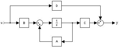
The most general state-space representation of a linear system with inputs, outputs and state variables is written in the following form:


where:
is called the "state vector", ; is called the "output vector", ; is called the "input (or control) vector", ; is the "state matrix", , is the "input matrix", , is the "output matrix", , is the "feedthrough (or feedforward) matrix" (in cases where the system model does not have a direct feedthrough, is the zero matrix), ,
-
 .
.
In this general formulation, all matrices are allowed to be time-variant (i.e., their elements can depend on time); however, in the common LTI case, matrices will be time invariant. The time variable
can be a "continuous" (e.g., ) or discrete (e.g., ). In the latter case, the time variable is usually indicated as . Hybrid systemHybrid system
A hybrid system is a dynamic system that exhibits both continuous and discrete dynamic behavior – a system that can both flow and jump...
s allow for time domains that have both continuous and discrete parts. Depending on the assumptions taken, the state-space model representation can assume the following forms:
| System type | State-space model |
| Continuous time-invariant |   |
| Continuous time-variant |   |
| Explicit discrete time-invariant |   |
| Explicit discrete time-variant |   |
| Laplace domain of continuous time-invariant |
  |
| Z-domain of discrete time-invariant |
  |
Example: Continuous-time LTI case
Stability and natural response characteristics of a continuous-time LTI system (i.e., linear with matrices that are constant with respect to time) can be studied from the eigenvalues of the matrix A. The stability of a time-invariant state-space model can be determined by looking at the system's transfer functionTransfer function
A transfer function is a mathematical representation, in terms of spatial or temporal frequency, of the relation between the input and output of a linear time-invariant system. With optical imaging devices, for example, it is the Fourier transform of the point spread function i.e...
in factored form. It will then look something like this:
The denominator of the transfer function is equal to the characteristic polynomial
Characteristic polynomial
In linear algebra, one associates a polynomial to every square matrix: its characteristic polynomial. This polynomial encodes several important properties of the matrix, most notably its eigenvalues, its determinant and its trace....
found by taking the determinant
Determinant
In linear algebra, the determinant is a value associated with a square matrix. It can be computed from the entries of the matrix by a specific arithmetic expression, while other ways to determine its value exist as well...
of
,

The roots of this polynomial (the eigenvalues) are the system transfer function's poles (i.e., the singularities
Mathematical singularity
In mathematics, a singularity is in general a point at which a given mathematical object is not defined, or a point of an exceptional set where it fails to be well-behaved in some particular way, such as differentiability...
where the transfer function's magnitude is unbounded). These poles can be used to analyze whether the system is asymptotically stable or marginally stable
Marginal stability
In the theory of dynamical systems, and control theory, a continuous linear time-invariant system is marginally stable if and only if the real part of every eigenvalue in the system's transfer-function is non-positive, and all eigenvalues with zero real value are simple roots...
. An alternative approach to determining stability, which does not involve calculating eigenvalues, is to analyze the system's Lyapunov stability
Lyapunov stability
Various types of stability may be discussed for the solutions of differential equations describing dynamical systems. The most important type is that concerning the stability of solutions near to a point of equilibrium. This may be discussed by the theory of Lyapunov...
.
The zeros found in the numerator of
can similarly be used to determine whether the system is minimum phaseMinimum phase
In control theory and signal processing, a linear, time-invariant system is said to be minimum-phase if the system and its inverse are causal and stable....
.
The system may still be input–output stable (see BIBO stable
BIBO stability
In electrical engineering, specifically signal processing and control theory, BIBO stability is a form of stability for linear signals and systems that take inputs. BIBO stands for Bounded-Input Bounded-Output...
) even though it is not internally stable. This may be the case if unstable poles are canceled out by zeros (i.e., if those singularities in the transfer function are removable).
Controllability
Thus, state controllability condition implies that it is possible – by admissible inputs – to steer the states from any initial value to any final value within some finite time window. A continuous time-invariant linear state-space model is controllable if and only ifIFF
IFF, Iff or iff may refer to:Technology/Science:* Identification friend or foe, an electronic radio-based identification system using transponders...
Where rank
Rank (linear algebra)
The column rank of a matrix A is the maximum number of linearly independent column vectors of A. The row rank of a matrix A is the maximum number of linearly independent row vectors of A...
is the number of linearly independent rows in a matrix.
Observability
Observability is a measure for how well internal states of a system can be inferred by knowledge of its external outputs. The observability and controllability of a system are mathematical duals (i.e., as controllability provides that an input is available that brings any initial state to any desired final state, observability provides that knowing an output trajectory provides enough information to predict the initial state of the system).A continuous time-invariant linear state-space model is observable if and only if
Transfer function
The "transfer functionTransfer function
A transfer function is a mathematical representation, in terms of spatial or temporal frequency, of the relation between the input and output of a linear time-invariant system. With optical imaging devices, for example, it is the Fourier transform of the point spread function i.e...
" of a continuous time-invariant linear state-space model can be derived in the following way:
First, taking the Laplace transform of
yields
Next, we simplify for
, givingand thus
Substituting for
in the output equation givingBecause the transfer function
Transfer function
A transfer function is a mathematical representation, in terms of spatial or temporal frequency, of the relation between the input and output of a linear time-invariant system. With optical imaging devices, for example, it is the Fourier transform of the point spread function i.e...
is defined as the ratio of the output to the input of a system, we takeand substitute the previous expression for
with respect to , givingClearly
must have by dimensionality, and thus has a total of elements.So for every input there are
transfer functions with one for each output.This is why the state-space representation can easily be the preferred choice for multiple-input, multiple-output (MIMO) systems.
Canonical realizations
Any given transfer function which is strictly properStrictly proper
In control theory, a strictly proper transfer function is a transfer function where the degree of the numerator is less than the degree of the denominator.-Example:...
can easily be transferred into state-space by the following approach (this example is for a 4-dimensional, single-input, single-output system)):
Given a transfer function, expand it to reveal all coefficients in both the numerator and denominator. This should result in the following form:
The coefficients can now be inserted directly into the state-space model by the following approach:
This state-space realization is called controllable canonical form because the resulting model is guaranteed to be controllable (i.e., because the control enters a chain of integrators, it has the ability to move every state).
The transfer function coefficients can also be used to construct another type of canonical form
This state-space realization is called observable canonical form because the resulting model is guaranteed to be observable (i.e., because the output exists from a chain of integrators, every state has an effect on the output).
Proper transfer functions
Transfer functions which are only properProper transfer function
In control theory, a proper transfer function is a transfer function in which the degree of the numerator does not exceed the degree of the denominator.-Example:...
(and not strictly proper
Strictly proper
In control theory, a strictly proper transfer function is a transfer function where the degree of the numerator is less than the degree of the denominator.-Example:...
) can also be realised quite easily. The trick here is to separate the transfer function into two parts: a strictly proper part and a constant.
The strictly proper transfer function can then be transformed into a canonical state space realization using techniques shown above. The state space realization of the constant is trivially
. Together we then get a state space realization with matrices A,B and C determined by the strictly proper part, and matrix D determined by the constant.Here is an example to clear things up a bit:
which yields the following controllable realization
Notice how the output also depends directly on the input. This is due to the
constant in the transfer function.Feedback
.Since the values of K are unrestricted the values can easily be negated for negative feedback
Negative feedback
Negative feedback occurs when the output of a system acts to oppose changes to the input of the system, with the result that the changes are attenuated. If the overall feedback of the system is negative, then the system will tend to be stable.- Overview :...
.
The presence of a negative sign (the common notation) is merely a notational one and its absence has no impact on the end results.


becomes


solving the output equation for
and substituting in the state equation results in

The advantage of this is that the eigenvalues of A can be controlled by setting K appropriately through eigendecomposition of
.This assumes that the closed-loop system is controllable
Controllability
Controllability is an important property of a control system, and the controllability property plays a crucial role in many control problems, such as stabilization of unstable systems by feedback, or optimal control....
or that the unstable eigenvalues of A can be made stable through appropriate choice of K.
Example
For a strictly proper system D equals zero. Another fairly common situation is when all states are outputs, i.e. y = x, which yields C = I, the Identity matrixIdentity matrix
In linear algebra, the identity matrix or unit matrix of size n is the n×n square matrix with ones on the main diagonal and zeros elsewhere. It is denoted by In, or simply by I if the size is immaterial or can be trivially determined by the context...
. This would then result in the simpler equations


This reduces the necessary eigendecomposition to just
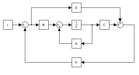
.Feedback with setpoint (reference) input
, can be added such that .

becomes


solving the output equation for
and substituting in the state equationresults in


One fairly common simplification to this system is removing D, which reduces the equations to


Moving object example
A classical linear system is that of one-dimensional movement of an object.The Newton's laws of motion
Newton's laws of motion
Newton's laws of motion are three physical laws that form the basis for classical mechanics. They describe the relationship between the forces acting on a body and its motion due to those forces...
for an object moving horizontally on a plane and attached to a wall with a spring
where
 is position;
  is velocity;
  is acceleration
 is an applied force
 is the viscous friction coefficient
 is the spring constant
 is the mass of the object
The state equation would then become
where
 represents the position of the object
 is the velocity of the object
 is the acceleration of the object
- the output
 is the position of the object
The controllability
Controllability
Controllability is an important property of a control system, and the controllability property plays a crucial role in many control problems, such as stabilization of unstable systems by feedback, or optimal control....
test is then
which has full rank for all
and .The observability
Observability
Observability, in control theory, is a measure for how well internal states of a system can be inferred by knowledge of its external outputs. The observability and controllability of a system are mathematical duals. The concept of observability was introduced by American-Hungarian scientist Rudolf E...
test is then
which also has full rank.
Therefore, this system is both controllable and observable.
Nonlinear systems
The more general form of a state space model can be written as two functions.The first is the state equation and the latter is the output equation.
If the function
is a linear combination of states and inputs then the equations can be written in matrix notation like above.The
argument to the functions can be dropped if the system is unforced (i.e., it has no inputs).Pendulum example
A classic nonlinear system is a simple unforced pendulumPendulum
A pendulum is a weight suspended from a pivot so that it can swing freely. When a pendulum is displaced from its resting equilibrium position, it is subject to a restoring force due to gravity that will accelerate it back toward the equilibrium position...
where
 is the angle of the pendulum with respect to the direction of gravity
 is the mass of the pendulum (pendulum rod's mass is assumed to be zero)
 is the gravitational acceleration
 is coefficient of friction at the pivot point
 is the radius of the pendulum (to the center of gravity of the mass
  )
)
The state equations are then
where
 is the angle of the pendulum
 is the rotational velocity of the pendulum
 is the rotational acceleration of the pendulum
Instead, the state equation can be written in the general form
The equilibrium
Mechanical equilibrium
A standard definition of static equilibrium is:This is a strict definition, and often the term "static equilibrium" is used in a more relaxed manner interchangeably with "mechanical equilibrium", as defined next....
/stationary point
Stationary point
In mathematics, particularly in calculus, a stationary point is an input to a function where the derivative is zero : where the function "stops" increasing or decreasing ....
s of a system are when
and so the equilibrium points of a pendulum are those that satisfyfor integers n.
Further reading
- Antsaklis, P.J. and Michel, A.N. 2007. A Linear Systems Primer, Birkhauser. (ISBN 978-0-8176-4434-50)
- Chen, Chi-Tsong 1999. Linear System Theory and Design, 3rd. ed., Oxford University Press (ISBN 0-19-511777-8)
- Khalil, Hassan K. 2001 Nonlinear Systems, 3rd. ed., Prentice Hall (ISBN 0-13-067389-7)
- Nise, Norman S. 2004. Control Systems Engineering, 4th ed., John Wiley & Sons, Inc. (ISBN 0-471-44577-0)
- Hinrichsen, Diederich and Pritchard, Anthony J. 2005. Mathematical Systems Theory I, Modelling, State Space Analysis, Stability and Robustness. Springer. (ISBN 978-3-540-44125-0)
- Sontag, Eduardo D. 1999. Mathematical Control Theory: Deterministic Finite Dimensional Systems. Second Edition. Springer. (ISBN 0-387-98489-5) (available free online)
- Friedland, Bernard. 2005. Control System Design: An Introduction to State Space Methods. Dover. (ISBN 0-486-44278-0).
- Zadeh, Lofti A. and Desoer, Charles A. 1979. Linear System Theory, Krieger Pub Co. (ISBN 978-0-88275-809-1)
On the applications of state space models in econometrics:
- Durbin, J. and S. Koopman (2001). Time series analysis by state space methods. Oxford University Press, Oxford.
See also
- Control engineeringControl engineeringControl engineering or Control systems engineering is the engineering discipline that applies control theory to design systems with predictable behaviors...
- Control theoryControl theoryControl theory is an interdisciplinary branch of engineering and mathematics that deals with the behavior of dynamical systems. The desired output of a system is called the reference...
- State observerState observerIn control theory, a state observer is a system that models a real system in order to provide an estimate of its internal state, given measurements of the input and output of the real system. It is typically a computer-implemented mathematical model....
- ObservabilityObservabilityObservability, in control theory, is a measure for how well internal states of a system can be inferred by knowledge of its external outputs. The observability and controllability of a system are mathematical duals. The concept of observability was introduced by American-Hungarian scientist Rudolf E...
- ControllabilityControllabilityControllability is an important property of a control system, and the controllability property plays a crucial role in many control problems, such as stabilization of unstable systems by feedback, or optimal control....
- DiscretizationDiscretizationIn mathematics, discretization concerns the process of transferring continuous models and equations into discrete counterparts. This process is usually carried out as a first step toward making them suitable for numerical evaluation and implementation on digital computers...
of state space models - Phase spacePhase spaceIn mathematics and physics, a phase space, introduced by Willard Gibbs in 1901, is a space in which all possible states of a system are represented, with each possible state of the system corresponding to one unique point in the phase space...
for information about phase state (like state space) in physics and mathematics. - State spaceState spaceIn the theory of discrete dynamical systems, a state space is a directed graph where each possible state of a dynamical system is represented by a vertex, and there is a directed edge from a to b if and only if ƒ = b where the function f defines the dynamical system.State spaces are...
for information about state space with discrete states in computer science. - State space (physics)State space (physics)In physics, a state space is a complex Hilbert space within which the possible instantaneous states of the system may be described by a unit vector. These state vectors, using Dirac's bra-ket notation, can often be treated as vectors and operated on using the rules of linear algebra...
for information about state space in physics.