

Quantization (signal processing)
Encyclopedia
Digital signal processing
Digital signal processing is concerned with the representation of discrete time signals by a sequence of numbers or symbols and the processing of these signals. Digital signal processing and analog signal processing are subfields of signal processing...
, is the process of mapping a large set of input values to a smaller set – such as rounding
Rounding
Rounding a numerical value means replacing it by another value that is approximately equal but has a shorter, simpler, or more explicit representation; for example, replacing $23.4476 with $23.45, or the fraction 312/937 with 1/3, or the expression √2 with 1.414.Rounding is often done on purpose to...
values to some unit of precision. A device or algorithmic function that performs quantization is called a quantizer. The error introduced by quantization is referred to as quantization error
Quantization error
In analog-to-digital conversion, the difference between the actual analog value and quantized digital value is called quantization error or quantization distortion. This error is either due to rounding or truncation...
or round-off error
Round-off error
A round-off error, also called rounding error, is the difference between the calculated approximation of a number and its exact mathematical value. Numerical analysis specifically tries to estimate this error when using approximation equations and/or algorithms, especially when using finitely many...
. Quantization is involved to some degree in nearly all digital signal processing, as the process of representing a signal in digital form ordinarily involves rounding. Quantization also forms the core of essentially all lossy compression algorithms.
Because quantization is a many-to-few mapping, it is an inherently non-linear and irreversible process (i.e., because the same output value is shared by multiple input values, it is impossible in general to recover the exact input value when given only the output value).
The set of possible input values may be infinitely large, and may possibly be continuous and therefore uncountable (such as the set of all real number
Real number
In mathematics, a real number is a value that represents a quantity along a continuum, such as -5 , 4/3 , 8.6 , √2 and π...
s, or all real numbers within some limited range). The set of possible output values may be finite or countably infinite
Countable set
In mathematics, a countable set is a set with the same cardinality as some subset of the set of natural numbers. A set that is not countable is called uncountable. The term was originated by Georg Cantor...
. The input and output sets involved in quantization can be defined in rather general way. For example, vector quantization
Vector quantization
Vector quantization is a classical quantization technique from signal processing which allows the modeling of probability density functions by the distribution of prototype vectors. It was originally used for data compression. It works by dividing a large set of points into groups having...
is the application of quantization to multi-dimensional (vector-valued) input data.
There are two substantially different classes of applications where quantization is used:
- The first type, which may simply be called rounding quantization, is the one employed for many applications, to enable the use of a simple approximate representation for some quantity that is to be measured and used in other calculations. This category includes the simple rounding approximations used in everyday arithmetic. This category also includes analog-to-digital conversion of a signal for a digital signal processing system (e.g., using a sound card of a personal computer to capture an audio signal) and the calculations performed within most digital filtering processes. Here the purpose is primarily to retain as much signal fidelity as possible while eliminating unnecessary precision and keeping the dynamic range of the signal within practical limits (to avoid signal clippingClipping (signal processing)Clipping is a form of distortion that limits a signal once it exceeds a threshold. Clipping may occur when a signal is recorded by a sensor that has constraints on the range of data it can measure, it can occur when a signal is digitized, or it can occur any other time an analog or digital signal...
or arithmetic overflowArithmetic overflowThe term arithmetic overflow or simply overflow has the following meanings.# In a computer, the condition that occurs when a calculation produces a result that is greater in magnitude than that which a given register or storage location can store or represent.# In a computer, the amount by which a...
). In such uses, substantial loss of signal fidelity is often unacceptable, and the design often centers around managing the approximation error to ensure that very little distortion is introduced. - The second type, which can be called rate–distortion optimized quantization, is encountered in source codingSource codingIn information theory, Shannon's source coding theorem establishes the limits to possible data compression, and the operational meaning of the Shannon entropy....
for "lossy" data compression algorithms, where the purpose is to manage distortion within the limits of the bit rate supported by a communication channel or storage medium. In this second setting, the amount of introduced distortion may be managed carefully by sophisticated techniques, and introducing some significant amount of distortion may be unavoidable. A quantizer designed for this purpose may be quite different and more elaborate in design than an ordinary rounding operation. It is in this domain that substantial rate–distortion theory analysis is likely to be applied. However, the same concepts actually apply in both use cases.
The analysis of quantization involves studying the amount of data (typically measured in digits or bits or bit rate) that is used to represent the output of the quantizer, and studying the loss of precision that is introduced by the quantization process (which is referred to as the distortion). The general field of such study of rate and distortion is known as rate–distortion theory.
Scalar quantization
The most common type of quantization is known as scalar quantization. Scalar quantization, typically denoted as , is the process of using a quantization function
  ( ) to map a scalar (one-dimensional) input value
  to a scalar output value
  . Scalar quantization can be as simple and intuitive as rounding
Rounding
Rounding a numerical value means replacing it by another value that is approximately equal but has a shorter, simpler, or more explicit representation; for example, replacing $23.4476 with $23.45, or the fraction 312/937 with 1/3, or the expression √2 with 1.414.Rounding is often done on purpose to...
high-precision numbers to the nearest integer, or to the nearest multiple of some other unit of precision (such as rounding a large monetary amount to the nearest thousand dollars). Scalar quantization of continuous-valued input data that is performed by an electronic sensor
Sensor
A sensor is a device that measures a physical quantity and converts it into a signal which can be read by an observer or by an instrument. For example, a mercury-in-glass thermometer converts the measured temperature into expansion and contraction of a liquid which can be read on a calibrated...
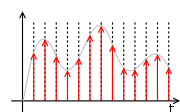
is referred to as analog-to-digital conversion. Analog-to-digital conversion often also involves sampling
Sampling (signal processing)
In signal processing, sampling is the reduction of a continuous signal to a discrete signal. A common example is the conversion of a sound wave to a sequence of samples ....
the signal periodically in time (e.g., at 44.1 kHz
Hertz
The hertz is the SI unit of frequency defined as the number of cycles per second of a periodic phenomenon. One of its most common uses is the description of the sine wave, particularly those used in radio and audio applications....
for CD
Compact Disc
The Compact Disc is an optical disc used to store digital data. It was originally developed to store and playback sound recordings exclusively, but later expanded to encompass data storage , write-once audio and data storage , rewritable media , Video Compact Discs , Super Video Compact Discs ,...
-quality audio signals).
Rounding example
As an example, roundingRounding
Rounding a numerical value means replacing it by another value that is approximately equal but has a shorter, simpler, or more explicit representation; for example, replacing $23.4476 with $23.45, or the fraction 312/937 with 1/3, or the expression √2 with 1.414.Rounding is often done on purpose to...
a real number
Real number
In mathematics, a real number is a value that represents a quantity along a continuum, such as -5 , 4/3 , 8.6 , √2 and π...
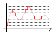
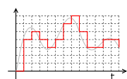
 to the nearest integer value forms a very basic type of quantizer – a uniform one. A typical (mid-tread) uniform quantizer with a quantization step size equal to some value
  can be expressed as
 ,
,where the function
 ( ) is the sign function
Sign function
In mathematics, the sign function is an odd mathematical function that extracts the sign of a real number. To avoid confusion with the sine function, this function is often called the signum function ....
(also known as the signum function).
For simple rounding to the nearest integer, the step size
 is equal to 1. With
  or with
  equal to any other integer value, this quantizer has real-valued inputs and integer-valued outputs, although this property is not a necessity – a quantizer may also have an integer input domain and may also have non-integer output values. The essential property of a quantizer is that it has a countable set of possible output values that has fewer members than the set of possible input values. The members of the set of output values may have integer, rational, or real values (or even other possible values as well, in general – such as vector values or complex number
Complex number
A complex number is a number consisting of a real part and an imaginary part. Complex numbers extend the idea of the one-dimensional number line to the two-dimensional complex plane by using the number line for the real part and adding a vertical axis to plot the imaginary part...
s).
When the quantization step size is small (relative to the variation in the signal being measured), it is relatively simple to show that the mean squared error
Mean squared error
In statistics, the mean squared error of an estimator is one of many ways to quantify the difference between values implied by a kernel density estimator and the true values of the quantity being estimated. MSE is a risk function, corresponding to the expected value of the squared error loss or...
produced by such a rounding operation will be approximately
 .
.Because the set of possible output values of a quantizer is countable, any quantizer can be decomposed into two distinct stages, which can be referred to as the classification stage (or forward quantization stage) and the reconstruction stage (or inverse quantization stage), where the classification stage maps the input value to an integer quantization index
 and the reconstruction stage maps the index
  to the reconstruction value
  that is the output approximation of the input value. For the example uniform quantizer described above, the forward quantization stage can be expressed as
 ,
,and the reconstruction stage for this example quantizer is simply
 .
.This decomposition is useful for the design and analysis of quantization behavior, and it illustrates how the quantized data can be communicated over a communication channel – a source encoder can perform the forward quantization stage and send the index information through a communication channel (possibly applying entropy coding techniques to the quantization indices), and a decoder can perform the reconstruction stage to produce the output approximation of the original input data. In more elaborate quantization designs, both the forward and inverse quantization stages may be substantially more complex. In general, the forward quantization stage may use any function that maps the input data to the integer space of the quantization index data, and the inverse quantization stage can conceptually (or literally) be a table look-up operation to map each quantization index to a corresponding reconstruction value. This two-stage decomposition applies equally well to vector
Vector quantization
Vector quantization is a classical quantization technique from signal processing which allows the modeling of probability density functions by the distribution of prototype vectors. It was originally used for data compression. It works by dividing a large set of points into groups having...
as well as scalar quantizers.
Mid-riser and mid-tread uniform quantizers
Most uniform quantizers for signed input data can be classified as being of one of two types: mid-riser and mid-tread. The terminology is based on what happens in the region around the value 0, and uses the analogy of viewing the input-output function of the quantizer as a stairwayStairway
Stairway, staircase, stairwell, flight of stairs, or simply stairs are names for a construction designed to bridge a large vertical distance by dividing it into smaller vertical distances, called steps...
. Mid-tread quantizers have a zero-valued reconstruction level (corresponding to a tread of a stairway), while mid-riser quantizers have a zero-valued classification threshold (corresponding to a riser
Stair riser
A stair riser is the near-vertical element in a set of stairs, forming the space between a step and the next. It is often slightly inclined from the vertical so that its top is closer than its base to the person climbing the stairs...
of a stairway).
The formulas for mid-tread uniform quantization are provided above.
The input-output formula for a mid-riser uniform quantizer is given by:
 ,
,where the classification rule is given by

and the reconstruction rule is
 .
.Note that mid-riser uniform quantizers do not have a zero output value – their minimum output magnitude is half the step size. When the input data can be modeled as a random variable
Random variable
In probability and statistics, a random variable or stochastic variable is, roughly speaking, a variable whose value results from a measurement on some type of random process. Formally, it is a function from a probability space, typically to the real numbers, which is measurable functionmeasurable...
with a probability density function
Probability density function
In probability theory, a probability density function , or density of a continuous random variable is a function that describes the relative likelihood for this random variable to occur at a given point. The probability for the random variable to fall within a particular region is given by the...
(pdf) that is smooth and symmetric around zero, mid-riser quantizers also always produce an output entropy of at least 1 bit per sample.
In contrast, mid-tread quantizers do have a zero output level, and can reach arbitrarily low bit rates per sample for input distributions that are symmetric and taper off at higher magnitudes. For some applications, having a zero output signal representation or supporting low output entropy may be a necessity. In such cases, using a mid-tread uniform quantizer may be appropriate while using a mid-riser one would not be.
In general, a mid-riser or mid-tread quantizer may not actually be a uniform quantizer – i.e., the size of the quantizer's classification intervals may not all be the same, or the spacing between its possible output values may not all be the same. The distinguishing characteristic of a mid-riser quantizer is that it has a classification threshold value that is exactly zero, and the distinguishing characteristic of a mid-tread quantizer is that is it has a reconstruction value that is exactly zero.
Another name for a mid-tread quantizer is dead-zone quantizer, and the classification region around the zero output value of such a quantizer is referred to as the dead zone. The dead zone can sometimes serve the same purpose as a noise gate
Noise gate
A Noise Gate or gate is an electronic device or software that is used to control the volume of an audio signal. In its most simple form, a noise gate allows a signal to pass through only when it is above a set threshold: the gate is 'open'. If the signal falls below the threshold no signal is...
or squelch
Squelch
In telecommunications, squelch is a circuit function that acts to suppress the audio output of a receiver in the absence of a sufficiently strong desired input signal.-Carrier squelch:...
function.
Granular distortion and overload distortion
Often the design of a quantizer involves supporting only a limited range of possible output values and performing clipping to limit the output to this range whenever the input exceeds the supported range. The error introduced by this clipping is referred to as overload distortion. Within the extreme limits of the supported range, the amount of spacing between the selectable output values of a quantizer is referred to as its granularity, and the error introduced by this spacing is referred to as granular distortion. It is common for the design of a quantizer to involve determining the proper balance between granular distortion and overload distortion. For a given supported number of possible output values, reducing the average granular distortion may involve increasing the average overload distortion, and vice-versa. A technique for controlling the amplitude of the signal (or, equivalently, the quantization step size ) to achieve the appropriate balance is the use of automatic gain control
Automatic gain control
Automatic gain control is an adaptive system found in many electronic devices. The average output signal level is fed back to adjust the gain to an appropriate level for a range of input signal levels...
(AGC). However, in some quantizer designs, the concepts of granular error and overload error may not apply (e.g., for a quantizer with a limited range of input data or with a countably infinite set of selectable output values).
The additive noise model for quantization error
A common assumption for the analysis of quantization errorQuantization error
In analog-to-digital conversion, the difference between the actual analog value and quantized digital value is called quantization error or quantization distortion. This error is either due to rounding or truncation...
is that it affects a signal processing system in a similar manner to that of additive white noise
White noise
White noise is a random signal with a flat power spectral density. In other words, the signal contains equal power within a fixed bandwidth at any center frequency...
– having negligible correlation with the signal and an approximately flat power spectral density. The additive noise model is commonly used for the analysis of quantization error effects in digital filtering systems, and it can be very useful in such analysis. It has been shown to be a valid model in cases of high resolution quantization (small
 relative to the signal strength) with smooth probability density functions. However, additive noise behaviour is not always a valid assumption, and care should be taken to avoid assuming that this model always applies. In actuality, the quantization error (for quantizers defined as described here) is deterministically related to the signal rather than being independent of it, and in some cases it can even cause limit cycles to appear in digital signal processing systems.
One way to ensure effective independence of the quantization error from the source signal is to perform dither
Dither
Dither is an intentionally applied form of noise used to randomize quantization error, preventing large-scale patterns such as color banding in images...
ed quantization (sometimes with noise shaping
Noise shaping
Noise shaping is a technique typically used in digital audio, image, and video processing, usually in combination with dithering, as part of the process of quantization or bit-depth reduction of a digital signal...
), which involves adding random (or pseudo-random) noise to the signal prior to quantization. This can sometimes be beneficial for such purposes as improving the subjective quality of the result, however it can increase the total quantity of error introduced by the quantization process.
Rate–distortion quantizer design
A scalar quantizer, which performs a quantization operation, can ordinarily be decomposed into two stages:- Classification: A process that classifies the input signal range into
 non-overlapping intervals
  , by defining
  boundary (decision) values
  , such that
  for
for  , with the extreme limits defined by
  and
and  . All the inputs
  that fall in a given interval range
  are associated with the same quantization index
  .
. - Reconstruction: Each interval
 is represented by a reconstruction value
  which implements the mapping
  .
.
These two stages together comprise the mathematical operation of
 .
.Entropy coding techniques can be applied to communicate the quantization indices from a source encoder that performs the classification stage to a decoder that performs the reconstruction stage. One way to do this is to associate each quantization index
 with a binary codeword
  . An important consideration is the number of bits used for each codeword, denoted here by
  .
.As a result, the design of an
 -level quantizer and an associated set of codewords for communicating its index values requires finding the values of
  ,
,  and
and  which optimally satisfy a selected set of design constraints such as the bit rate
  and distortion
  .
.Assuming that an information source
 produces random variables
  with an associated probability density function
Probability density function
In probability theory, a probability density function , or density of a continuous random variable is a function that describes the relative likelihood for this random variable to occur at a given point. The probability for the random variable to fall within a particular region is given by the...
 , the probability
  that the random variable falls within a particular quantization interval
  is given by
 .
.The resulting bit rate
 , in units of average bits per quantized value, for this quantizer can be derived as follows:
 .
.If it is assumed that distortion is measured by mean squared error
Mean squared error
In statistics, the mean squared error of an estimator is one of many ways to quantify the difference between values implied by a kernel density estimator and the true values of the quantity being estimated. MSE is a risk function, corresponding to the expected value of the squared error loss or...
, the distortion D, is given by:
 .
.Note that other distortion measures can also be considered, although mean squared error is a popular one.
A key observation is that rate
 depends on the decision boundaries
  and the codeword lengths
  , whereas the distortion
  depends on the decision boundaries
  and the reconstruction levels
  .
.After defining these two performance metrics for the quantizer, a typical Rate–Distortion formulation for a quantizer design problem can be expressed in one of two ways:
- Given a maximum distortion constraint
 , minimize the bit rate
- Given a maximum bit rate constraint
 , minimize the distortion
Often the solution to these problems can be equivalently (or approximately) expressed and solved by converting the formulation to the unconstrained problem

where the Lagrange multiplier
 is a non-negative constant that establishes the appropriate balance between rate and distortion. Solving the unconstrained problem is equivalent to finding a point on the convex hull
Convex hull
In mathematics, the convex hull or convex envelope for a set of points X in a real vector space V is the minimal convex set containing X....
of the family of solutions to an equivalent constrained formulation of the problem. However, finding a solution – especially a closed-form
Closed-form expression
In mathematics, an expression is said to be a closed-form expression if it can be expressed analytically in terms of a bounded number of certain "well-known" functions...
solution – to any of these three problem formulations can be difficult. Solutions that do not require multi-dimensional iterative optimization techniques have been published for only three probability distribution functions: the uniform
Uniform distribution (continuous)
In probability theory and statistics, the continuous uniform distribution or rectangular distribution is a family of probability distributions such that for each member of the family, all intervals of the same length on the distribution's support are equally probable. The support is defined by...
, exponential
Exponential distribution
In probability theory and statistics, the exponential distribution is a family of continuous probability distributions. It describes the time between events in a Poisson process, i.e...
, and Laplacian distributions. Iterative optimization approaches can be used to find solutions in other cases.
Note that the reconstruction values
 affect only the distortion – they do not affect the bit rate – and that each individual
  makes a separate contribution
  to the total distortion as shown below:
where

This observation can be used to ease the analysis – given the set of
 values, the value of each
  can be optimized separately to minimize its contribution to the distortion
  .
.For the mean-square error distortion criterion, it can be easily shown that the optimal set of reconstruction values
 is given by setting the reconstruction value
  within each interval
  to the conditional expected value (also referred to as the centroid
Centroid
In geometry, the centroid, geometric center, or barycenter of a plane figure or two-dimensional shape X is the intersection of all straight lines that divide X into two parts of equal moment about the line. Informally, it is the "average" of all points of X...
) within the interval, as given by:
 .
.The use of sufficiently well-designed entropy coding techniques can result in the use of a bit rate that is close to the true information content of the indices
 , such that effectively
and therefore

The use of this approximation can allow the entropy coding design problem to be separated from the design of the quantizer itself. Modern entropy coding techniques such as arithmetic coding
Arithmetic coding
Arithmetic coding is a form of variable-length entropy encoding used in lossless data compression. Normally, a string of characters such as the words "hello there" is represented using a fixed number of bits per character, as in the ASCII code...
can achieve bit rates that are very close to the true entropy of a source, given a set of known (or adaptively estimated) probabilities
 .
.In some designs, rather than optimizing for a particular number of classification regions
 , the quantizer design problem may include optimization of the value of
  as well. For some probabilistic source models, the best performance may be achieved when
  approaches infinity.
Neglecting the entropy constraint: Lloyd–Max quantization
In the above formulation, if the bit rate constraint is neglected by setting equal to 0, or equivalently if it is assumed that a fixed-length code (FLC) will be used to represent the quantized data instead of a variable-length code
Variable-length code
In coding theory a variable-length code is a code which maps source symbols to a variable number of bits.Variable-length codes can allow sources to be compressed and decompressed with zero error and still be read back symbol by symbol...
(or some other entropy coding technology such as arithmetic coding
Arithmetic coding
Arithmetic coding is a form of variable-length entropy encoding used in lossless data compression. Normally, a string of characters such as the words "hello there" is represented using a fixed number of bits per character, as in the ASCII code...
that is better than an FLC in the rate–distortion sense), the optimization problem reduces to minimization of distortion
 alone.
The indices produced by an
 -level quantizer can be coded using a fixed-length code using
  bits/symbol. For example when
  256 levels, the FLC bit rate
  is 8 bits/symbol. For this reason, such a quantizer has sometimes been called an 8-bit quantizer. However using an FLC eliminates the compression improvement that can be obtained by use of better entropy coding.
Assuming an FLC with
 levels, the Rate–Distortion minimization problem can be reduced to distortion minimization alone.
The reduced problem can be stated as follows: given a source
 with pdf
Probability density function
In probability theory, a probability density function , or density of a continuous random variable is a function that describes the relative likelihood for this random variable to occur at a given point. The probability for the random variable to fall within a particular region is given by the...
 and the constraint that the quantizer must use only
  classification regions, find the decision boundaries
  and reconstruction levels
  to minimize the resulting distortion
Finding an optimal solution to the above problem results in a quantizer sometimes called a MMSQE (minimum mean-square quantization error) solution, and the resulting pdf-optimized (non-uniform) quantizer is referred to as a Lloyd–Max quantizer, named after two people who independently developed iterative methods to solve the two sets of simultaneous equations resulting from
 and
and  , as follows:
 ,
,which places each threshold at the mid-point between each pair of reconstruction values, and

which places each reconstruction value at the centroid (conditional expected value) of its associated classification interval.
Lloyd's Method I algorithm
Lloyd's algorithm
In computer science and electrical engineering, Lloyd's algorithm, also known as Voronoi iteration or relaxation, is an algorithm for grouping data points into a given number of categories, used for k-means clustering....
, originally described in 1957, can be generalized in a straighforward way for application to vector
Vector quantization
Vector quantization is a classical quantization technique from signal processing which allows the modeling of probability density functions by the distribution of prototype vectors. It was originally used for data compression. It works by dividing a large set of points into groups having...
data. This generalization results in the Linde–Buzo–Gray (LBG) or k-means classifier optimization methods. Moreover, the technique can be further generalized in a straightforward way to also include an entropy constraint for vector data.
Uniform quantization and the 6 dB/bit approximation
The Lloyd–Max quantizer is actually a uniform quantizer when the input pdfProbability density function
In probability theory, a probability density function , or density of a continuous random variable is a function that describes the relative likelihood for this random variable to occur at a given point. The probability for the random variable to fall within a particular region is given by the...
is uniformly distributed over the range
 . However, for a source that does not have a uniform distribution, the minimum-distortion quantizer may not be a uniform quantizer.
The analysis of a uniform quantizer applied to a uniformly distributed source can be summarized in what follows:
A symmetric source X can be modelled with
 , for
, for  and 0 elsewhere.
The step size
 and the signal to quantization noise ratio (SQNR) of the quantizer is
SQNR
 .
.For a fixed-length code using
 bits,
bits,  , resulting in
SQNR
 dB,
dB,or approximately 6 dB per bit. For example, for
 =8 bits,
  =256 levels and SQNR = 8*6 = 48 dB; and for
  =16 bits,
  =65536 and SQNR = 16*6 = 96 dB. The property of 6 dB improvement in SQNR for each exta bit used in quantization is a well-known figure of merit. However, it must be used with care: this derivation is only for a uniform quantizer applied to a uniform source.
For other source pdfs and other quantizer designs, the SQNR may be somewhat different than predicted by 6 dB/bit, depending on the type of pdf, the type of source, the type of quantizer, and the bit rate range of operation.
However, it is common to assume that for many sources, the slope of a quantizer SQNR function can be approximated as 6 dB/bit when operating at a sufficiently high bit rate. At asymptotically high bit rates, cutting the step size in half increases the bit rate by approximately 1 bit per sample (because 1 bit is needed to indicate whether the value is in the left or right half of the prior double-sized interval) and reduces the mean squared error by a factor of 4 (i.e., 6 dB) based on the
 approximation.
At asymptotically high bit rates, the 6 dB/bit approximation is supported for many source pdfs by rigorous theoretical analysis. Moreover, the structure of the optimal scalar quantizer (in the rate–distortion sense) approaches that of a uniform quantizer under these conditions.
Companding quantizers
Companded quantizationCompanding
In telecommunication, signal processing, and thermodynamics, companding is a method of mitigating the detrimental effects of a channel with limited dynamic range...
is the combination of three functional building blocks – namely, a (continuous-domain) signal dynamic range compressor, a limited-range uniform quantizer, and a (continuous-domain) signal dynamic range expander that basically inverts the compressor function. This type of quantization is frequently used in older speech telephony systems. The compander function of the compressor is key to the performance of such a quantization system. In principle, the compressor function can be designed to exactly map the boundaries of the optimal intervals of any desired scalar quantizer function to the equal-size intervals used by the uniform quantizer and similarly the expander function can exactly map the uniform quantizer reconstruction values to any arbitrary reconstruction values. Thus, with arbitrary compressor and expander functions, any possible non-uniform scalar quantizer can be equivalently implemented as a companded quantizer. In practice, companders are designed to operate according to relatively-simple dynamic range compressor functions that are designed to be suitable for implementation using simple analog electronic circuits. The two most popular compander functions used for telecommunications are the A-law
A-law algorithm
An A-law algorithm is a standard companding algorithm, used in European digital communications systems to optimize, i.e., modify, the dynamic range of an analog signal for digitizing.It is similar to the μ-law algorithm used in North America and Japan....
and μ-law functions.