
Mathematics of Sudoku
Encyclopedia
The class
of Sudoku
puzzle
s consists of a partially completed row-column grid of cells partitioned into N regions each of size N cells, to be filled in using a prescribed set of N distinct symbols (typically the numbers {1, ..., N}), so that each row, column and region contains exactly one of each element of the set. The puzzle can be investigated using mathematics
.
and permutation group theory
, augmented by the dexterous application of programming tools.
There are many Sudoku variants, (partially) characterized by the size (N) and shape of their regions. For classic Sudoku, N=9 and the regions are 3x3 squares (called blocks or boxes). A rectangular Sudoku uses rectangular regions of row-column dimension R×C. For R×1 (and 1×C), i.e. where the region is a row or column, Sudoku becomes a Latin square
.
Other Sudoku variants also exist, such as those with irregularly-shaped regions or with additional constraints (hypercube) or different (Samunamupure) constraint types. See Sudoku - Variants for a discussion of variants and Sudoku terms and jargon for an expanded listing.
The mathematics of Sudoku is a relatively new area of exploration, mirroring the popularity of Sudoku itself. NP-complete
ness was documented late 2002 , enumeration results began appearing in May 2005 .
In contrast with the two main mathematical approaches of Sudoku mentioned above, an approach resting on mathematical logic and dealing with the resolution of the puzzles from the viewpoint of a player has recently been proposed in Denis Berthier's book "The Hidden Logic of Sudoku". This formalizes certain mathematical symmetries of the game and elicits resolution rules based on them, such as "hidden xy-chains".
. For n=3 (classical Sudoku), however, this result is of little relevance: algorithm
s such as Dancing Links
can solve puzzles in fractions of a second.
Solving Sudoku puzzles can be expressed as a graph coloring
problem. Consider the 9 × 9 = 32 × 32 case. The aim of the puzzle in its standard form is to construct a proper 9-coloring of a particular graph, given a partial 9-coloring. The graph in question has 81 vertices, one vertex for each cell of the grid. The vertices can be labeled with the ordered pairs
(x, y), where x and y are integers between 1 and 9. In this case, two distinct vertices labeled by (x, y) and (x′, y′) are joined by an edge if and only if:
The puzzle is then completed by assigning an integer between 1 and 9 to each vertex, in such a way that vertices that are joined by an edge do not have the same integer assigned to them.
A valid Sudoku solution grid is also a Latin square
. There are significantly fewer valid Sudoku solution grids than Latin squares because Sudoku imposes the additional regional constraint. Nonetheless, the number of valid Sudoku solution grids for the standard 9×9 grid was calculated by Bertram Felgenhauer and Frazer Jarvis in 2005 to be 6,670,903,752,021,072,936,960 . This number is equal to 9! × 722 × 27 × 27,704,267,971, the last factor of which is prime
. The result was derived through logic and brute force computation
. Russell and Jarvis also showed that when symmetries were taken into account, there were 5,472,730,538 solutions . The number of valid Sudoku solution grids for the 16×16 derivation is not known.
The maximum number of givens that can be provided while still not rendering the solution unique, regardless of variation, is four short of a full grid; if two instances of two numbers each are missing and the cells they are to occupy are the corners of an orthogonal rectangle, and exactly two of these cells are within one region, there are two ways the numbers can be added. The inverse of this—the fewest givens that render a solution unique—is an unsolved problem
, although the lowest number yet found for the standard variation without a symmetry constraint is 17, a number of which have been found by Japanese puzzle enthusiasts , and 18 with the givens in rotationally symmetric cells.
s the (addition- or) multiplication table
s (Cayley table
s) of finite groups can be used to construct Sudokus and related tables of numbers. Namely, one has to take subgroups and quotient group
s into account:
Take for example the group of pairs, adding each component separately modulo some
  .
.
By omitting one of the components, we suddenly find ourselves in (and this mapping is obviously compatible with the respective additions, i.e. it is a group homomorphism).
One also says that the latter is a quotient group
of the former, because some once different elements become equal in the new group.
However, it is also a subgroup
, because we can simply fill the missing component with to get back to
  .
.
Under this view, we write down the example :
:
Each Sudoku region looks the same on the second component (namely like the subgroup ), because these are added regardless of the first one.
On the other hand, the first components are equal in each block, and if we imagine each block as one cell, these first components show the same pattern (namely the quotient group ).
).
As already outlined in the article of Latin square
s, this really is a Latin square of order .
.
Now, to yield a Sudoku, let us permute the rows (or equivalently the columns) in such a way, that each block is redistributed exactly once into each block - for example order them .
.
This of course preserves the Latin square property. Furthermore, in each block the lines have distinct first component by construction
and each line in a block has distinct entries via the second component, because the blocks' second components originally formed a Latin square of order (from the subgroup
  ).
).
Thus we really get a Sudoku (Rename the pairs to numbers 1...9 if you wish)! With the example and the row permutation above, we yield:
For this method to work, one generally does not need a product of two equally-sized groups. A so-called short exact sequence
of finite groups
of appropriate size already does the job! Try for example the group with quotient- and subgroup
  .
.
It seems clear (already from enumeration arguments), that not all Sudokus can be generated this way!
Horizontally adjacent blocks constitute a band (the vertical equivalent is called a stack).
A proper puzzle has a unique solution. The constraint 'each digit appears in each row, column and region' is called the One Rule.
See basic terms or the List of Sudoku terms and jargon for an expanded list of terminology.
es tiled in a 6x6 grid. The following notation is used for discussing this variant. RxC denotes a rectangular region with R rows and C columns. The implied grid configuration has R blocks per band (C blocks per stack), C×R bands×stacks and grid dimensions NxN, with N = R · C. Puzzles of size NxN, where N is prime can only be tiled with irregular N-ominoes. Each NxN grid can be tiled multiple ways with N-ominoes. Before enumerating the number of solutions to a Sudoku grid of size NxN, it is necessary to determine how many N-omino tilings exist for a given size (including the standard square tilings, as well as the rectangular tilings).
The size ordering of Sudoku puzzle can be used to define an integer series, e.g. for square Sudoku, the integer series of possible solutions .
Sudoku with square NxN regions are more symmetrical than immediately obvious from the One Rule. Each row and column intersects N regions and shares N cells with each. The number of bands and stacks also equals N. Rectangular Sudoku do not have these properties. The "3x3" Sudoku is additionally unique: N is also the number of row-column-region constraints from the One Rule (i.e. there are N=3 types of units).
See the List of Sudoku terms and jargon for an expanded list and classification of variants.
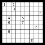
The number of solutions depends on the grid dimensions, rules applied and the definition of distinct solutions. For the 3×3 region grid, the conventions for labeling the rows, columns, blocks (boxes) are as shown. Bands are numbered top to bottom, stacks left to right. By extension the labeling scheme applies to any rectangular Sudoku grid.
Term labels for box-row and box-column triplets are also shown.
The {a, b, c} notation also reflects that fact a triplet is a subset
of the allowed digits. For regions of arbitrary dimension, the related object is known as a minicol(umn) or minirow.
and equivalence classes for the partial grid solutions were identified, the completions of the lower two bands were constructed and counted for each equivalence class. Summing completions over the equivalence classes, weighted by class size, gives the total number of solutions as 6,670,903,752,021,072,936,960 (6.67×10²¹). The value was subsequently confirmed numerous times independently. The Algorithm details section (below) describes the method.
These operations define a symmetry relation between equivalent grids.
Excluding relabeling, and with respect to the 81 grid cell values, the operations form a subgroup
of the symmetric group
S81, of order 3!8×2 = 3359232.
It has been shown that any fixed operation on the tiles that always translates a valid Sudoku grid into another valid grid can be generated from the operations listed above (excluding relabeling).
. The number of essentially different solutions is then the number of orbits, which can be computed using Burnside's lemma
. The Burnside fixed points are solutions that differ only by relabeling. Using this technique, Jarvis/Russell computed the number of essentially different (symmetrically distinct) solutions as
5,472,730,538.
The paper 'Enumerating possible Sudoku grids' , by Felgenhauer and Jarvis, describes the calculation.
Since then, enumeration results for many Sudoku variants have been calculated: these are summarised below.
The standard 3×3 calculation can be carried out in less than a second on a PC. The 3×4 (= 4×3) problem is much harder and took 2568 hours to solve, split over several computers.

where bR,C is the number of ways of completing a Sudoku band of R horizontally adjacent R×C boxes. Petersen's algorithm , as implemented by Silver , is currently the fastest known technique for exact evaluation of these bR,C.
The band counts for problems whose full Sudoku grid-count is unknown are listed below. As in the previous section, "Dimensions" are those of the regions.
The expression for the 4×C case is:

where:
All Sudokus remain valid (no repeated numbers in any row, column or region) under the action of the Sudoku preserving symmetries (see also Jarvis ). Some Sudokus are special in that some operations merely have the effect of relabelling the digits; several of these are enumerated below.
Further calculations of this ilk combine to show that the number of essentially different Sudoku grids is 5,472,730,538, for example as demonstrated by Jarvis / Russell and verified by Pettersen . Similar methods have been applied to the 2x3 case, where Jarvis / Russell showed that there are 49 essentially different grids (see also the article by Bailey, Cameron and Connelly ), to the 2x4 case, where Russell showed that there are 1,673,187 essentially different grids (verified by Pettersen ), and to the 2x5 case where Pettersen showed that there are 4,743,933,602,050,718 essentially different grids (not verified).
 Additional constraints (here, on 3×3 Sudokus) lead to a smaller minimum number of clues.
A variant on Miyuki Misawa's web site replaces sums with relations: the clues are symbols =, < and > showing the relative values of (some but not all) adjacent region sums. She demonstrates an example with only eight relations. It is not known whether this is the best possible.
'Enumerating possible Sudoku grids' .
The methods and algorithms used are very straight forward and provide a practical introduction to several mathematical concepts. The development is presented here for those wishing to explore these topics.
The strategy begins by analyzing the permutations of the top band used in valid solutions. Once the Band1 symmetries
and equivalence class for the partial solutions are identified, the completions of the lower two bands are constructed and counted for each equivalence class. Summing the completions over the equivalence classes gives the total number of solutions as 6,670,903,752,021,072,936,960 (c. 6.67×10²¹).
(This expression may be generalized to any R×3 box band variant. (Pettersen ). Thus B2 contributes 56 × 63 permutations.
The permutations for Band1 are 9! × 56 × 66 = 9! × 2612736 ~ 9.48 × 10¹¹.
(Note: Conditional combinations becomes an increasingly difficult as the computation progresses through the grid. At this point the impact is minimal.)
Case 0: No Overlap. The choices for the triplets can be determined by elimination.
r21 can't be r11 or r12 so it must be = r13; r31 must be = r12 etc.
The Case 0 diagram shows this configuration, where the pink cells are triplet values that can be arranged in any order within the triplet.
Each triplet has 3! = 6 permutations. The 6 triplets contribute 66 permutations.
Case 3: 3 Digits Match: triplet r21 = r12. The same logic as case 0 applies, but with a different triplet usage.
Triplet r22 must be = r13, etc.
The number of permutations is again 66. (Felgenhauer/Jarvis call the cases 0 and 3 the pure match case.
Case 1: 1 Match for r21 from r12
In the Case 1 diagram, B1 cells show canonical values, which are color coded to show their row-wise distribution in B2 triplets. Colors reflect distribution but not location or values. For this case: the B2 top row triplet (r21) has 1 value from B1 middle triplet, the other colorings can now be deduced. E.g. the B2 bottom row triplet (r23) coloring is forced by r21: the other 2 B1 middle values must go to bottom, etc. Fill in the number of B2 options for each color, 3..1, beginning top left. The B3 color coding is omitted since the B3 choices are row-wise determined by B1, B2. B3 always contributes 3! permutations per row triplet, or 63 for the block.
For B2, the triplet values can appear in any position, so a 3! permutation factor still applies, for each triplet. However,
since some of the values were paired relative to their origin, using the raw option counts would overcount the number of permutations, due to interchangeability within the pairing. The option counts need to be divided by the permuted size of their grouping (2), here 2!.= 2 (See n Choose k) The pair in each row cancels the 2s for the B2 option counts, leaving a B2 contribution of 33 × 63. The B2×B3 combined contribution is 33 × 66.
Case 2: 2 Matches for r21 from r12. The same logic as case 1 applies, but with the B2 option count column groupings reversed. Case 3 also contributes 33×66 permutations.
Totaling the 4 cases for Band1 B1..B3 gives
9! × 2 × (33 + 1) × 66 = 9! 56 × 66 permutations.
A symmetry in mathematics
is an operation that preserves a quality of an object. For a Sudoku solution grid, a symmetry is a transformation whose result is also a solution grid. The following symmetries apply independently for the top band:
Combined, the symmetries give 9! × 65 = 362880 × 7776 equivalent permutations for each Band1 solution.
A symmetry defines an equivalence relation
, here, between the solutions, and partitions
the solutions into a set of equivalence classes. The Band1 row, column and block symmetries divide the 56*6^6 permutations into (not less than) 336 (56×6) equivalence classes with (up to) 65 permutations in each, and 9! relabeling permutations for each class. (Min/Max caveats apply since some permutations may not yield distinct elements due to relabeling.)
Since the solution for any member of an equivalence class can be generated from the solution of any other member, we only need to enumerate the solutions for a single member in order to enumerate all solutions over all classes. Let
The total number of solutions N is then:
Counting symmetry partitions valid Band1 permutations into classes that place the same completion constraints on lower bands; all members of a band counting symmetry equivalence class must have the same number of grid completions since the completion constraints are equivalent. Counting symmetry constraints are identified by the Band1 column triplets (a column value set, no implied element order). Using band counting symmetry, a minimal generating set of 44 equivalence classes was established.
Note, while column triplets are used to construct and identify the equivalence classes, the class members themselves are the valid Band1 permutations: class size (Sb.z) reflects column triplet permutations compatible with the One Rule solution requirements. Counting symmetry is a completion property and applies only to a partial grid (band or stack). Solution symmetry for preserving solutions can be applied to either partial grids (bands, stacks) or full grid solutions. Lastly note, counting symmetry is more restrictive than simple numeric completion count equality: two (distinct) bands belong to the same counting symmetry equivalence class only if they impose equivalent completion constraints.
The Band1 (65) symmetries divide the (56×66) Band1 valid permutations into (not less than) 336 (56×6) equivalence classes with (up to) 6^5 permutations each.
The not less than and up to caveats are necessary, since some combinations of the transformations may not produce distinct results, when relabeling is required (see below). Consequently some equivalence classes may contain less than 65 distinct permutations and the theoretical minimum number of classes may not be achieved.
Each of the valid Band1 permutations can be expanded (completed) into a specific number of solutions with the Band2,3 permutations. By virtue of their similarity, each member of an equivalence class will have the same number of completions. Consequently we only need to construct the solutions for one member of each equivalence class and then multiply the number of solutions by the size of the equivalence class.
We are still left with the task of identifying and calculating the size of each equivalence class. Further progress requires the dexterous application of computational techniques to catalogue (classify and count) the permutations into equivalence classes.
Felgenhauer/Jarvis catalogued the Band1 permutations using lexicographical order
ed IDs based on the ordered digits from blocks B2,3. Block 1 uses a canonical digit assignment and is not needed for a unique ID. Equivalence class identification and linkage uses the lowest ID within the class.
Application of the (2×62) B2,3 symmetry permutations produces 36288 (28×64) equivalence classes, each of size 72. Since the size is fixed, the computation only needs to find the 36288 equivalence class IDs. (Note: in this case,
for any Band1 permutation, applying these permutations to achieve the lowest ID provides an index to the associated equivalence class.)
Application of the rest of the block, column and row symmetries provided further reduction, i.e. allocation of the 36288 IDs into fewer, larger equivalence classes.
When the B1 canonical labeling is lost through a transformation, the result is relabeled to the canonical B1 usage and then catalogued under this ID. This approach generated 416 equivalence classes, somewhat less effective than the theoretical 336 minimum limit for a full reduction.
Application of counting symmetry patterns for duplicate paired digits achieved reduction to 174 and then to 71 equivalence classes. The introduction of equivalence classes based on band counting symmetry (subsequent to Felgenhauer/Jarvis by Russell ) reduced the equivalence classes to a minimum generating set of 44.
The diversity of the ~2.6×10⁶, 56×66 Band1 permutations can be reduced to a set of 44 Band1 equivalence classes. Each of the 44 equivalence classes can be expanded to millions of distinct full solutions, but the entire solution space has a common origin in these 44. The 44 equivalence classes play a central role in other enumeration approaches as well, and speculation will return to the characteristics of the 44 classes when puzzle properties are explored later.
For each of the Band1 equivalence classes, all possible Band2,3 solutions need to be enumerated. An outer Band1 loop iterates over the 44 equivalence classes. In the inner loop, all lower band completions for each of the Band1 equivalence class are found and counted.
The computation required for the lower band solution search can be minimised by the same type of symmetry application used for Band1. There are 6! (720) permutations for the 6 values in column 1 of Band2,3. Applying the lower band (2) and row within band (6×6) permutations creates 10 equivalence classes of size 72. At this point, completing 10 sets of solutions for the remaining 48 cells with a recursive descent, backtracking
algorithm is feasible with 2 GHz class PC so further simplification is not required to carry out the enumeration.
Using this approach, the number of ways of filling in a blank Sudoku grid was shown in May 2005 (original announcement ) to be 6,670,903,752,021,072,936,960 (6.67×10²¹).
The paper 'Enumerating possible Sudoku grids' by Felgenhauer and Jarvis, describes the calculation.
The result, as confirmed by Russell , also contains the distribution of solution counts for the 44 equivalence classes. The listed values are before application of the 9! factor for labeling and the two 72 factors (722 = 5184) for each of Stack 2,3 and Band2,3 permutations. The number of completions for each class is consistently on the order of 100,000,000, while the number of Band1 permutations covered by each class however varies from 4 – 3240. Within this wide size range, there are clearly two clusters. Ranked by size, the lower 33 classes average ~400 permutations/class, while the upper 11 average ~2100. The disparity in consistency between the distributions for size and number of completions or the separation into two clusters by size is yet to be examined.
 The largest rectangular orthogonal "hole" (region with no clues) in a proper sudoku is believed to be a rectangle of 30 cells (a 5 x 6 rectangular area).
One such example is the following with 22 clues:
 The largest total number of empty groups (rows, columns, and squares) in a sudoku is believed to be nine. One example is the following; a sudoku which has 3 empty squares, 3 empty rows, and 3 empty columns and gives 22 clues.
Notice that if this sudoku is rotated 180 degrees, and the clues relabeled with the permutation (123456789) -> (987654321), it returns to the same sudoku. Expressed another way, this sudoku has the property that every 180 degree rotational pair of clues (a, b) follows the rule (a) + (b) = 10.
Since this sudoku is automorphic, so too its solution grid must be automorphic. Furthermore, every cell which is solved has a symmetrical partner which is solved with the same technique (and the pair would take the form a + b = 10).
In this example the automorphism is easy to identify, but in general automorphism is not always obvious. There are several types of transformations of a sudoku, and therefore automorphism can take several different forms too. Among the population of all sudoku grids, those that are automorphic are rare. They are considered interesting because of their intrinsic mathematical symmetry.
Class (set theory)
In set theory and its applications throughout mathematics, a class is a collection of sets which can be unambiguously defined by a property that all its members share. The precise definition of "class" depends on foundational context...
of Sudoku
Sudoku
is a logic-based, combinatorial number-placement puzzle. The objective is to fill a 9×9 grid with digits so that each column, each row, and each of the nine 3×3 sub-grids that compose the grid contains all of the digits from 1 to 9...
puzzle
Puzzle
A puzzle is a problem or enigma that tests the ingenuity of the solver. In a basic puzzle, one is intended to put together pieces in a logical way in order to come up with the desired solution...
s consists of a partially completed row-column grid of cells partitioned into N regions each of size N cells, to be filled in using a prescribed set of N distinct symbols (typically the numbers {1, ..., N}), so that each row, column and region contains exactly one of each element of the set. The puzzle can be investigated using mathematics
Mathematics
Mathematics is the study of quantity, space, structure, and change. Mathematicians seek out patterns and formulate new conjectures. Mathematicians resolve the truth or falsity of conjectures by mathematical proofs, which are arguments sufficient to convince other mathematicians of their validity...
.
Overview
The mathematical analysis of Sudoku falls into two main areas: analyzing the properties of a) completed grids and b) puzzles. Grid analysis has largely focused on counting (enumerating) possible solutions for different variants. Puzzle analysis centers on the initial given values. The techniques used in either are largely the same: combinatoricsCombinatorics
Combinatorics is a branch of mathematics concerning the study of finite or countable discrete structures. Aspects of combinatorics include counting the structures of a given kind and size , deciding when certain criteria can be met, and constructing and analyzing objects meeting the criteria ,...
and permutation group theory
Permutation group
In mathematics, a permutation group is a group G whose elements are permutations of a given set M, and whose group operation is the composition of permutations in G ; the relationship is often written as...
, augmented by the dexterous application of programming tools.
There are many Sudoku variants, (partially) characterized by the size (N) and shape of their regions. For classic Sudoku, N=9 and the regions are 3x3 squares (called blocks or boxes). A rectangular Sudoku uses rectangular regions of row-column dimension R×C. For R×1 (and 1×C), i.e. where the region is a row or column, Sudoku becomes a Latin square
Latin square
In combinatorics and in experimental design, a Latin square is an n × n array filled with n different symbols, each occurring exactly once in each row and exactly once in each column...
.
Other Sudoku variants also exist, such as those with irregularly-shaped regions or with additional constraints (hypercube) or different (Samunamupure) constraint types. See Sudoku - Variants for a discussion of variants and Sudoku terms and jargon for an expanded listing.
The mathematics of Sudoku is a relatively new area of exploration, mirroring the popularity of Sudoku itself. NP-complete
NP-complete
In computational complexity theory, the complexity class NP-complete is a class of decision problems. A decision problem L is NP-complete if it is in the set of NP problems so that any given solution to the decision problem can be verified in polynomial time, and also in the set of NP-hard...
ness was documented late 2002 , enumeration results began appearing in May 2005 .
In contrast with the two main mathematical approaches of Sudoku mentioned above, an approach resting on mathematical logic and dealing with the resolution of the puzzles from the viewpoint of a player has recently been proposed in Denis Berthier's book "The Hidden Logic of Sudoku". This formalizes certain mathematical symmetries of the game and elicits resolution rules based on them, such as "hidden xy-chains".
Mathematical context
The general problem of solving Sudoku puzzles on n2 × n2 boards of n × n blocks is known to be NP-completeNP-complete
In computational complexity theory, the complexity class NP-complete is a class of decision problems. A decision problem L is NP-complete if it is in the set of NP problems so that any given solution to the decision problem can be verified in polynomial time, and also in the set of NP-hard...
. For n=3 (classical Sudoku), however, this result is of little relevance: algorithm
Algorithm
In mathematics and computer science, an algorithm is an effective method expressed as a finite list of well-defined instructions for calculating a function. Algorithms are used for calculation, data processing, and automated reasoning...
s such as Dancing Links
Dancing Links
In computer science, Dancing Links, also known as DLX, is the technique suggested by Donald Knuth to efficiently implement his Algorithm X. Algorithm X is a recursive, nondeterministic, depth-first, backtracking algorithm that finds all solutions to the exact cover problem...
can solve puzzles in fractions of a second.
Solving Sudoku puzzles can be expressed as a graph coloring
Graph coloring
In graph theory, graph coloring is a special case of graph labeling; it is an assignment of labels traditionally called "colors" to elements of a graph subject to certain constraints. In its simplest form, it is a way of coloring the vertices of a graph such that no two adjacent vertices share the...
problem. Consider the 9 × 9 = 32 × 32 case. The aim of the puzzle in its standard form is to construct a proper 9-coloring of a particular graph, given a partial 9-coloring. The graph in question has 81 vertices, one vertex for each cell of the grid. The vertices can be labeled with the ordered pairs
(x, y), where x and y are integers between 1 and 9. In this case, two distinct vertices labeled by (x, y) and (x′, y′) are joined by an edge if and only if:
- x = x′ (same column) or,
- y = y′ (same row) or,
- ⌈ x/3 ⌉ = ⌈ x′/3 ⌉ and ⌈ y/3 ⌉ = ⌈ y′/3 ⌉ (same 3 × 3 cell)
The puzzle is then completed by assigning an integer between 1 and 9 to each vertex, in such a way that vertices that are joined by an edge do not have the same integer assigned to them.
A valid Sudoku solution grid is also a Latin square
Latin square
In combinatorics and in experimental design, a Latin square is an n × n array filled with n different symbols, each occurring exactly once in each row and exactly once in each column...
. There are significantly fewer valid Sudoku solution grids than Latin squares because Sudoku imposes the additional regional constraint. Nonetheless, the number of valid Sudoku solution grids for the standard 9×9 grid was calculated by Bertram Felgenhauer and Frazer Jarvis in 2005 to be 6,670,903,752,021,072,936,960 . This number is equal to 9! × 722 × 27 × 27,704,267,971, the last factor of which is prime
Prime number
A prime number is a natural number greater than 1 that has no positive divisors other than 1 and itself. A natural number greater than 1 that is not a prime number is called a composite number. For example 5 is prime, as only 1 and 5 divide it, whereas 6 is composite, since it has the divisors 2...
. The result was derived through logic and brute force computation
Computation
Computation is defined as any type of calculation. Also defined as use of computer technology in Information processing.Computation is a process following a well-defined model understood and expressed in an algorithm, protocol, network topology, etc...
. Russell and Jarvis also showed that when symmetries were taken into account, there were 5,472,730,538 solutions . The number of valid Sudoku solution grids for the 16×16 derivation is not known.
The maximum number of givens that can be provided while still not rendering the solution unique, regardless of variation, is four short of a full grid; if two instances of two numbers each are missing and the cells they are to occupy are the corners of an orthogonal rectangle, and exactly two of these cells are within one region, there are two ways the numbers can be added. The inverse of this—the fewest givens that render a solution unique—is an unsolved problem
Unsolved problems in mathematics
This article lists some unsolved problems in mathematics. See individual articles for details and sources.- Millennium Prize Problems :Of the seven Millennium Prize Problems set by the Clay Mathematics Institute, six have yet to be solved:* P versus NP...
, although the lowest number yet found for the standard variation without a symmetry constraint is 17, a number of which have been found by Japanese puzzle enthusiasts , and 18 with the givens in rotationally symmetric cells.
Sudokus from group tables
As in the case of Latin squareLatin square
In combinatorics and in experimental design, a Latin square is an n × n array filled with n different symbols, each occurring exactly once in each row and exactly once in each column...
s the (addition- or) multiplication table
Multiplication table
In mathematics, a multiplication table is a mathematical table used to define a multiplication operation for an algebraic system....
s (Cayley table
Cayley table
A Cayley table, after the 19th century British mathematician Arthur Cayley, describes the structure of a finite group by arranging all the possible products of all the group's elements in a square table reminiscent of an addition or multiplication table...
s) of finite groups can be used to construct Sudokus and related tables of numbers. Namely, one has to take subgroups and quotient group
Quotient group
In mathematics, specifically group theory, a quotient group is a group obtained by identifying together elements of a larger group using an equivalence relation...
s into account:
Take for example
the group of pairs, adding each component separately modulo some .By omitting one of the components, we suddenly find ourselves in
(and this mapping is obviously compatible with the respective additions, i.e. it is a group homomorphism).One also says that the latter is a quotient group
Quotient group
In mathematics, specifically group theory, a quotient group is a group obtained by identifying together elements of a larger group using an equivalence relation...
of the former, because some once different elements become equal in the new group.
However, it is also a subgroup
Subgroup
In group theory, given a group G under a binary operation *, a subset H of G is called a subgroup of G if H also forms a group under the operation *. More precisely, H is a subgroup of G if the restriction of * to H x H is a group operation on H...
, because we can simply fill the missing component with
to get back to .Under this view, we write down the example
:Each Sudoku region looks the same on the second component (namely like the subgroup
), because these are added regardless of the first one.On the other hand, the first components are equal in each block, and if we imagine each block as one cell, these first components show the same pattern (namely the quotient group
).As already outlined in the article of Latin square
Latin square
In combinatorics and in experimental design, a Latin square is an n × n array filled with n different symbols, each occurring exactly once in each row and exactly once in each column...
s, this really is a Latin square of order
.Now, to yield a Sudoku, let us permute the rows (or equivalently the columns) in such a way, that each block is redistributed exactly once into each block - for example order them
.This of course preserves the Latin square property. Furthermore, in each block the lines have distinct first component by construction
and each line in a block has distinct entries via the second component, because the blocks' second components originally formed a Latin square of order
(from the subgroup ).Thus we really get a Sudoku (Rename the pairs to numbers 1...9 if you wish)! With the example and the row permutation above, we yield:
For this method to work, one generally does not need a product of two equally-sized groups. A so-called short exact sequence
Exact sequence
An exact sequence is a concept in mathematics, especially in homological algebra and other applications of abelian category theory, as well as in differential geometry and group theory...
of finite groups
of appropriate size already does the job! Try for example the group
with quotient- and subgroup .It seems clear (already from enumeration arguments), that not all Sudokus can be generated this way!
Terminology
A puzzle is a partially completed grid. The initial puzzle values are known as givens or clues. The regions are also called boxes or blocks. The use of the term square is generally avoided because of ambiguity.Horizontally adjacent blocks constitute a band (the vertical equivalent is called a stack).
A proper puzzle has a unique solution. The constraint 'each digit appears in each row, column and region' is called the One Rule.
See basic terms or the List of Sudoku terms and jargon for an expanded list of terminology.
Variants
Sudoku regions are polyominoes. Although the classic "3x3" Sudoku is made of square nonominoes, it is possible to apply the rules of Sudoku to puzzles of other sizes – the 2x2 and 4x4 square puzzles, for example. Only N2xN2 Sudoku puzzles can be tiled with square polyominoes. Another popular variant is made of rectangular regions – for example, 2x3 hexominoHexomino
A hexomino is a polyomino of order 6, that is, a polygon in the plane made of 6 equal-sized squares connected edge-to-edge. The name of this type of figure is formed with the prefix hex-. When rotations and reflections are not considered to be distinct shapes, there are 35 different free hexominoes...
es tiled in a 6x6 grid. The following notation is used for discussing this variant. RxC denotes a rectangular region with R rows and C columns. The implied grid configuration has R blocks per band (C blocks per stack), C×R bands×stacks and grid dimensions NxN, with N = R · C. Puzzles of size NxN, where N is prime can only be tiled with irregular N-ominoes. Each NxN grid can be tiled multiple ways with N-ominoes. Before enumerating the number of solutions to a Sudoku grid of size NxN, it is necessary to determine how many N-omino tilings exist for a given size (including the standard square tilings, as well as the rectangular tilings).
The size ordering of Sudoku puzzle can be used to define an integer series, e.g. for square Sudoku, the integer series of possible solutions .
Sudoku with square NxN regions are more symmetrical than immediately obvious from the One Rule. Each row and column intersects N regions and shares N cells with each. The number of bands and stacks also equals N. Rectangular Sudoku do not have these properties. The "3x3" Sudoku is additionally unique: N is also the number of row-column-region constraints from the One Rule (i.e. there are N=3 types of units).
See the List of Sudoku terms and jargon for an expanded list and classification of variants.
Definition of terms and labels
Let- s be a solution to a Sudoku grid with specific dimensions, satisfying the One Rule constraints
- S = {s}, be the set of all solutions
- |S|, the cardinality of S, is the number of elements in S, i.e. the number of solutions, also known as the size of S.
The number of solutions depends on the grid dimensions, rules applied and the definition of distinct solutions. For the 3×3 region grid, the conventions for labeling the rows, columns, blocks (boxes) are as shown. Bands are numbered top to bottom, stacks left to right. By extension the labeling scheme applies to any rectangular Sudoku grid.
Term labels for box-row and box-column triplets are also shown.
- triplet - an unordered combination of 3 values used in a box-row (or box-column), e.g. a triplet = {3, 5, 7} means the values 3, 5, 7 occur in a box-row (column) without specifying their location order. A triplet has 6 (3!) ordered permutations. By convention, triplet values are represented by their ordered digits. Triplet objects are labeled as:
- rBR, identifies a row triplet for box B and (grid) row R, e.g. r56 is the triplet for box 5, row 6, using the grid row label.
- cBC, identifies similarly a column triplet for box B and (grid) column row C.
The {a, b, c} notation also reflects that fact a triplet is a subset
Subset
In mathematics, especially in set theory, a set A is a subset of a set B if A is "contained" inside B. A and B may coincide. The relationship of one set being a subset of another is called inclusion or sometimes containment...
of the allowed digits. For regions of arbitrary dimension, the related object is known as a minicol(umn) or minirow.
Enumerating Sudoku solutions
The answer to the question 'How many Sudokus are there?' depends on the definition of when similar solutions are considered different.Enumerating all possible Sudoku solutions
For the enumeration of all possible solutions, two solutions are considered distinct if any of their corresponding (81) cell values differ. Symmetry relations between similar solutions are ignored., e.g. the rotations of a solution are considered distinct. Symmetries play a significant role in the enumeration strategy, but not in the count of all possible solutions.Enumerating the Sudoku 9×9 grid solutions directly
The first approach taken historically to enumerate Sudoku solutions ('Enumerating possible Sudoku grids' by Felgenhauer and Jarvis) was to analyze the permutations of the top band used in valid solutions. Once the Band1 symmetriesSymmetry in mathematics
Symmetry occurs not only in geometry, but also in other branches of mathematics. It is actually the same as invariance: the property that something does not change under a set of transformations....
and equivalence classes for the partial grid solutions were identified, the completions of the lower two bands were constructed and counted for each equivalence class. Summing completions over the equivalence classes, weighted by class size, gives the total number of solutions as 6,670,903,752,021,072,936,960 (6.67×10²¹). The value was subsequently confirmed numerous times independently. The Algorithm details section (below) describes the method.
Enumeration using band generation
A second enumeration technique based on band generation was later developed that is significantly less computationally intensive.Enumerating essentially different Sudoku solutions
Two valid grids are essentially the same if one can be derived from the other.Sudoku preserving symmetries
The following operations always translate a valid Sudoku grid into another valid grid: (values represent permutations for classic Sudoku)- Relabeling symbols (9!)
- Band permutations (3!)
- Row permutations within a band (3!3)
- Stack permutations (3!)
- Column permutations within a stack (3!3)
- Reflection, transposition and rotation (2). (Given any transposition or quarter-turn rotation in conjunction with the above permutations, any combination of reflections, transpositions and rotations can be produced, so these operations only contribute a factor of 2.)
These operations define a symmetry relation between equivalent grids.
Excluding relabeling, and with respect to the 81 grid cell values, the operations form a subgroup
Subgroup
In group theory, given a group G under a binary operation *, a subset H of G is called a subgroup of G if H also forms a group under the operation *. More precisely, H is a subgroup of G if the restriction of * to H x H is a group operation on H...
of the symmetric group
Symmetric group
In mathematics, the symmetric group Sn on a finite set of n symbols is the group whose elements are all the permutations of the n symbols, and whose group operation is the composition of such permutations, which are treated as bijective functions from the set of symbols to itself...
S81, of order 3!8×2 = 3359232.
It has been shown that any fixed operation on the tiles that always translates a valid Sudoku grid into another valid grid can be generated from the operations listed above (excluding relabeling).
Identifying distinct solutions with Burnside's Lemma
For a solution, the set of equivalent solutions which can be reached using these operations (excluding relabeling), form an orbit of the symmetric groupSymmetric group
In mathematics, the symmetric group Sn on a finite set of n symbols is the group whose elements are all the permutations of the n symbols, and whose group operation is the composition of such permutations, which are treated as bijective functions from the set of symbols to itself...
. The number of essentially different solutions is then the number of orbits, which can be computed using Burnside's lemma
Burnside's lemma
Burnside's lemma, sometimes also called Burnside's counting theorem, the Cauchy-Frobenius lemma or the orbit-counting theorem, is a result in group theory which is often useful in taking account of symmetry when counting mathematical objects. Its various eponyms include William Burnside, George...
. The Burnside fixed points are solutions that differ only by relabeling. Using this technique, Jarvis/Russell computed the number of essentially different (symmetrically distinct) solutions as
5,472,730,538.
Enumeration results
The number of ways of filling in a blank Sudoku grid was shown in May 2005 to be 6,670,903,752,021,072,936,960 (~6.67×10²¹) (original announcement ).The paper 'Enumerating possible Sudoku grids' , by Felgenhauer and Jarvis, describes the calculation.
Since then, enumeration results for many Sudoku variants have been calculated: these are summarised below.
Sudoku with rectangular regions
In the table, "Dimensions" are those of the regions (e.g. 3x3 in normal Sudoku). The "Rel Err" column indicates how a simple approximation, using the generalised method of Kevin Kilfoil , compares to the true grid count: it is an underestimate in all cases evaluated so far.| Dimensions | Nr Grids | Attribution | Verified? | Rel Err |
|---|---|---|---|---|
| 1x? | see Latin squares | n/a | ||
| 2×2 | 288 | various | Yes | -11.1% |
| 2×3 | 28200960 = c. 2.8×10⁷ | Pettersen | Yes | -5.88% |
| 2×4 | 29136487207403520 = c. 2.9×10¹⁶ | Russell | Yes | -1.91% |
| 2×5 | 1903816047972624930994913280000 = c. 1.9×1030 | Pettersen | Yes | -0.375% |
| 2×6 | 38296278920738107863746324732012492486187417600000 = c. 3.8×1049 | Pettersen | No | -0.238% |
| 3×3 | 6670903752021072936960 = c. 6.7×10²¹ | Felgenhauer/Jarvis | Yes | -0.207% |
| 3×4 | 81171437193104932746936103027318645818654720000 = c. 8.1×1046 | Pettersen / Silver | No | -0.132% |
| 3×5 | unknown, estimated c. 3.5086×1084 | Silver | n/a | |
| 4×4 | unknown, estimated c. 5.9584×1098 | Silver | n/a | |
| 4×5 | unknown, estimated c. 3.1764×10175 | Silver | n/a | |
| 5×5 | unknown, estimated c. 4.3648×10308 | Silver / Pettersen | n/a | |
The standard 3×3 calculation can be carried out in less than a second on a PC. The 3×4 (= 4×3) problem is much harder and took 2568 hours to solve, split over several computers.
Sudoku bands
For large (R,C), the method of Kevin Kilfoil (generalised method:) is used to estimate the number of grid completions. The method asserts that the Sudoku row and column constraints are, to first approximation, conditionally independent given the box constraint. Omitting a little algebra, this gives the Kilfoil-Silver-Pettersen formula:where bR,C is the number of ways of completing a Sudoku band of R horizontally adjacent R×C boxes. Petersen's algorithm , as implemented by Silver , is currently the fastest known technique for exact evaluation of these bR,C.
The band counts for problems whose full Sudoku grid-count is unknown are listed below. As in the previous section, "Dimensions" are those of the regions.
| Dimensions | Nr Bands | Attribution | Verified? |
|---|---|---|---|
| 2×C | (2C)! (C!)2 | (obvious result) | Yes |
| 3×C | 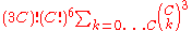 |
Pettersen | Yes |
| 4×C | (long expression: see below) | Pettersen | Yes |
| 4×4 | 16! × 4!12 × 1273431960 = c. 9.7304×1038 | Silver | Yes |
| 4×5 | 20! × 5!12 × 879491145024 = c. 1.9078×1055 | Russell | Yes |
| 4×6 | 24! × 6!12 × 677542845061056 = c. 8.1589×1072 | Russell | Yes |
| 4×7 | 28! × 7!12 × 563690747238465024 = c. 4.6169×1091 | Russell | Yes |
| (calculations up to 4×100 have been performed by Silver , but are not listed here) | |||
| 5×3 | 15! × 3!20 × 324408987992064 = c. 1.5510×1042 | Silver | Yes# |
| 5×4 | 20! × 4!20 × 518910423730214314176 = c. 5.0751×1066 | Silver | Yes# |
| 5×5 | 25! × 5!20 × 1165037550432885119709241344 = c. 6.9280×1093 | Pettersen / Silver | No |
| 5×6 | 30! × 6!20 × 3261734691836217181002772823310336 = c. 1.2127×10123 | Pettersen / Silver | No |
| 5×7 | 35! × 7!20 × 10664509989209199533282539525535793414144 = c. 1.2325×10154 | Pettersen / Silver | No |
| 5×8 | 40! × 8!20 × 39119312409010825966116046645368393936122855616 = c. 4.1157×10186 | Pettersen / Silver | No |
| 5×9 | 45! × 9!20 × 156805448016006165940259131378329076911634037242834944 = c. 2.9406×10220 | Pettersen / Silver | No |
| 5×10 | 50! × 10!20 × 674431748701227492664421138490224315931126734765581948747776 = c. 3.2157×10255 | Pettersen / Silver | No |
- # : same author, different method
The expression for the 4×C case is:
where:
- the outer summand is taken over all a,b,c such that 0<=a,b,c and a+b+c=2C
- the inner summand is taken over all k12,k13,k14,k23,k24,k34 ≥ 0 such that
- k12,k34 ≤ a and
- k13,k24 ≤ b and
- k14,k23 ≤ c and
- k12+k13+k14 = a-k12+k23+k24 = b-k13+c-k23+k34 = c-k14+b-k24+a-k34 = C
Sudoku with additional constraints
The following are all restrictions of 3x3 Sudokus. The type names have not been standardised: click on the attribution links to see the definitions.| Type | Nr Grids | Attribution | Verified? |
|---|---|---|---|
| 3doku | 104015259648 | Stertenbrink | Yes |
| Disjoint Groups | 201105135151764480 | Russell | Yes |
| Hypercube | 37739520 | Stertenbrink | Yes |
| Magic Sudoku | 5971968 | Stertenbrink | Yes |
| Sudoku X | 55613393399531520 | Russell | Yes |
| NRC Sudoku | 6337174388428800 | Brouwer | Yes |
All Sudokus remain valid (no repeated numbers in any row, column or region) under the action of the Sudoku preserving symmetries (see also Jarvis ). Some Sudokus are special in that some operations merely have the effect of relabelling the digits; several of these are enumerated below.
| Transformation | Nr Grids | Verified? |
|---|---|---|
| Transposition | 10980179804160 | Indirectly |
| Quarter Turn | 4737761280 | Indirectly |
| Half Turn | 56425064693760 | Indirectly |
| Band cycling | 5384326348800 | Indirectly |
| Within-band row cycling | 39007939461120 | Indirectly |
Further calculations of this ilk combine to show that the number of essentially different Sudoku grids is 5,472,730,538, for example as demonstrated by Jarvis / Russell and verified by Pettersen . Similar methods have been applied to the 2x3 case, where Jarvis / Russell showed that there are 49 essentially different grids (see also the article by Bailey, Cameron and Connelly ), to the 2x4 case, where Russell showed that there are 1,673,187 essentially different grids (verified by Pettersen ), and to the 2x5 case where Pettersen showed that there are 4,743,933,602,050,718 essentially different grids (not verified).
Minimum number of givens
Proper puzzles have a unique solution. An irreducible puzzle (or minimal puzzle) is a proper puzzle from which no givens can be removed leaving it a proper puzzle (with a single solution). It is possible to construct minimal puzzles with different numbers of givens. This section discusses the minimum number of givens for proper puzzles.Ordinary Sudoku
The lowest known is 17 givens in general Sudoku, or 18 when the positions of the givens are constrained to be half-turn rotationally symmetric. It is conjectured that these are the best possible, evidence for which stems from extensive randomised searching:- Gordon RoyleGordon RoyleGordon F. Royle is a Professor at the School of Mathematics and Statistics at The University of Western Australia. He is well known for his research into the mathematics of Sudoku and his search for the Sudoku puzzle with the smallest number of entries that has a unique solution.-See...
has compiled a list of 48826 17-clue puzzles , no two of which are isomorphic. None of these was isomorphic to a symmetric puzzle, nor contained a 16-clue puzzle. - The most fruitful set of clue positions, in terms of number of distinct 17-clue puzzles they admit, from Royle's list have been exhaustively searched for 17-clue puzzles. All 36 puzzles found by this process were already in Royle's list. All 34 puzzles on the next most fruitful set of clue positions were also in Royle's list.
- The most fruitful solution grids (in the same sense) have been exhaustively searched for 16-clue puzzles using CHECKER with no success. This includes one, "strangely familiar" , grid that yields exactly 29 different 17-clue puzzles, all of which had already been discovered by Royle's random search technique (suggesting once again that Royle's list of 17s is close to complete).
- A distributed computingDistributed computingDistributed computing is a field of computer science that studies distributed systems. A distributed system consists of multiple autonomous computers that communicate through a computer network. The computers interact with each other in order to achieve a common goal...
project, Sudoku@Vtaiwan, seeks to resolve the 16-clue problem.
Sudoku with additional constraints
- 3doku: no results for this variant
- Disjoint Groups: some 12-clue puzzles have been demonstrated by Glenn Fowler. Later also 11-clue puzzles are found. It is not known if this is the best possible.
- Hypercube: various 8-clue puzzles (the best possible) have been demonstrated by Guenter Stertenbrink.
- Magic Sudoku: a 7-clue example has been provided by Guenter Stertenbrink. It is not known if this is the best possible.
- Sudoku X: a list of 1167 12-clue puzzles has been collected by Ruud van der Werf. It is not known if this is the best possible.
- NRC Sudoku: an 11-clue example has been provided by Andries Brouwer. It is not known if this is the best possible.
- 2-Quasi-Magic Sudoku: a 4-clue example has been provided by Tony Forbes. It is suspected that this is the best possible.
Sudoku with irregular regions
"Du-sum-oh" (a.k.a. "geometry number place") puzzles replace the 3×3 (or R×C) regions of Sudoku with irregular shapes of a fixed size. Bob Harris has proved that it is always possible to create N-1 clue du-sum-ohs on an N×N grid, and has constructed several examples. Johan de Ruiter has proved that for any N>3 there exist polyomino tilings that can not be turned into a Sudoku puzzle with N irregular shapes of size N.Sum number place ("Killer Sudoku")
In sum number place (Samunamupure), the regions are of irregular shape and various sizes. The usual constraints of no repeated value in any row, column or region apply. The clues are given as sums of values within regions (e.g. a 4-cell region with sum 10 must consist of values 1,2,3,4 in some order). The minimum number of clues for Samunamupure is not known, nor even conjectured.A variant on Miyuki Misawa's web site replaces sums with relations: the clues are symbols =, < and > showing the relative values of (some but not all) adjacent region sums. She demonstrates an example with only eight relations. It is not known whether this is the best possible.
Method and algorithm details for the 9×9 grid direct enumeration
The approach described here was the historically first strategy employed to enumerate the Sudoku 9×9 grid solutions, as published by Felgenhauer and Jarvis in'Enumerating possible Sudoku grids' .
The methods and algorithms used are very straight forward and provide a practical introduction to several mathematical concepts. The development is presented here for those wishing to explore these topics.
The strategy begins by analyzing the permutations of the top band used in valid solutions. Once the Band1 symmetries
Symmetry in mathematics
Symmetry occurs not only in geometry, but also in other branches of mathematics. It is actually the same as invariance: the property that something does not change under a set of transformations....
and equivalence class for the partial solutions are identified, the completions of the lower two bands are constructed and counted for each equivalence class. Summing the completions over the equivalence classes gives the total number of solutions as 6,670,903,752,021,072,936,960 (c. 6.67×10²¹).
Counting the top band permutations
The Band1 algorithm proceeds as follows:- Choose a canonical labeling of the digits by assigning values for B1, e.g.
1 2 3

4 5 6

7 8 9
- Compute the rest of the Band1 permutations relative to the B1 canonical choice.
- Compute the permutations of B2 by partitioningPartition of a setIn mathematics, a partition of a set X is a division of X into non-overlapping and non-empty "parts" or "blocks" or "cells" that cover all of X...
the B1 cell values over the B2 row triplets. From the triplet combinations compute the B2 permutations. There are k=0..3 ways to choose the:
- Compute the permutations of B2 by partitioning
- B1 r11 values for B2 r22, the rest must go to r23,
- B1 r12 values for B2 r23, the rest must go to r21,
- B1 r13 values for B2 r21, the rest must go to r22, i.e.
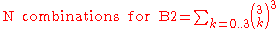
(This expression may be generalized to any R×3 box band variant. (Pettersen ). Thus B2 contributes 56 × 63 permutations.
- The choices for B3 triplets are row-wise determined by the B1 B2 row triplets. B3 always contributes 63 permutations.
The permutations for Band1 are 9! × 56 × 66 = 9! × 2612736 ~ 9.48 × 10¹¹.
Band1 permutation details
The permutations of B1 are the number of ways to relabel the 9 digits, 9! = 362880. Counting the permutations for B2 is more complicated, because the choices for B2 depend on the values in B1. (This is a visual representation of the expression given above.) The conditional calculation needs a branch (sub-calculation) for each alternative. Fortunately, there are just 4 cases for the top B2 triplet (r21): it contains either 0, 1, 2, or 3 of the digits from the B1 middle row triplet(r12). Once this B2 top row choice is made, the rest of the B2 combinations are fixed. The Band1 row triplet labels are shown on the right.(Note: Conditional combinations becomes an increasingly difficult as the computation progresses through the grid. At this point the impact is minimal.)
Case 0: No Overlap. The choices for the triplets can be determined by elimination.
r21 can't be r11 or r12 so it must be = r13; r31 must be = r12 etc.
The Case 0 diagram shows this configuration, where the pink cells are triplet values that can be arranged in any order within the triplet.
Each triplet has 3! = 6 permutations. The 6 triplets contribute 66 permutations.
Case 3: 3 Digits Match: triplet r21 = r12. The same logic as case 0 applies, but with a different triplet usage.
Triplet r22 must be = r13, etc.
The number of permutations is again 66. (Felgenhauer/Jarvis call the cases 0 and 3 the pure match case.
Case 1: 1 Match for r21 from r12
In the Case 1 diagram, B1 cells show canonical values, which are color coded to show their row-wise distribution in B2 triplets. Colors reflect distribution but not location or values. For this case: the B2 top row triplet (r21) has 1 value from B1 middle triplet, the other colorings can now be deduced. E.g. the B2 bottom row triplet (r23) coloring is forced by r21: the other 2 B1 middle values must go to bottom, etc. Fill in the number of B2 options for each color, 3..1, beginning top left. The B3 color coding is omitted since the B3 choices are row-wise determined by B1, B2. B3 always contributes 3! permutations per row triplet, or 63 for the block.
For B2, the triplet values can appear in any position, so a 3! permutation factor still applies, for each triplet. However,
since some of the values were paired relative to their origin, using the raw option counts would overcount the number of permutations, due to interchangeability within the pairing. The option counts need to be divided by the permuted size of their grouping (2), here 2!.= 2 (See n Choose k) The pair in each row cancels the 2s for the B2 option counts, leaving a B2 contribution of 33 × 63. The B2×B3 combined contribution is 33 × 66.
Case 2: 2 Matches for r21 from r12. The same logic as case 1 applies, but with the B2 option count column groupings reversed. Case 3 also contributes 33×66 permutations.
Totaling the 4 cases for Band1 B1..B3 gives
9! × 2 × (33 + 1) × 66 = 9! 56 × 66 permutations.
Band1 symmetries and equivalence classes
Symmetries are used to reduce the computational effort to enumerate the Band1 permutations.A symmetry in mathematics
Symmetry in mathematics
Symmetry occurs not only in geometry, but also in other branches of mathematics. It is actually the same as invariance: the property that something does not change under a set of transformations....
is an operation that preserves a quality of an object. For a Sudoku solution grid, a symmetry is a transformation whose result is also a solution grid. The following symmetries apply independently for the top band:
- Block B1 values may be relabeled, giving 9! permutations
- Blocks B1..3 may be interchanged, with 3!=6 permutations
- Rows 1..3 may be interchanged, with 3!=6 permutations
- Within each block, the 3 columns may be interchanged, giving 63 permutations.
Combined, the symmetries give 9! × 65 = 362880 × 7776 equivalent permutations for each Band1 solution.
A symmetry defines an equivalence relation
Equivalence relation
In mathematics, an equivalence relation is a relation that, loosely speaking, partitions a set so that every element of the set is a member of one and only one cell of the partition. Two elements of the set are considered equivalent if and only if they are elements of the same cell...
, here, between the solutions, and partitions
Partition of a set
In mathematics, a partition of a set X is a division of X into non-overlapping and non-empty "parts" or "blocks" or "cells" that cover all of X...
the solutions into a set of equivalence classes. The Band1 row, column and block symmetries divide the 56*6^6 permutations into (not less than) 336 (56×6) equivalence classes with (up to) 65 permutations in each, and 9! relabeling permutations for each class. (Min/Max caveats apply since some permutations may not yield distinct elements due to relabeling.)
Since the solution for any member of an equivalence class can be generated from the solution of any other member, we only need to enumerate the solutions for a single member in order to enumerate all solutions over all classes. Let
- sb : be a valid permutation of the top band
- Sb = [sb] : be an equivalence class, relative to sb and some equivalence relationEquivalence relationIn mathematics, an equivalence relation is a relation that, loosely speaking, partitions a set so that every element of the set is a member of one and only one cell of the partition. Two elements of the set are considered equivalent if and only if they are elements of the same cell...
- Sb.z = |Sb| : the size of Sb, be the number of sb elements (permutations) in [sb]
- Sb.n : be the number of Band2,3 completions for (any) sb in Sb
- {Sb} : be the set of all Sb equivalence classes relative to the equivalence relationEquivalence relationIn mathematics, an equivalence relation is a relation that, loosely speaking, partitions a set so that every element of the set is a member of one and only one cell of the partition. Two elements of the set are considered equivalent if and only if they are elements of the same cell...
- {Sb}.z = |{Sb}| : be the number of equivalence classes
The total number of solutions N is then:
Solution and counting permutation symmetry
The Band1 symmetries (above) are solution permutation symmetries defined so that a permuted solution is also a solution. For the purpose of enumerating solutions, a counting symmetry for grid completion can be used to define band equivalence classes that yield a minimal number of classes.Counting symmetry partitions valid Band1 permutations into classes that place the same completion constraints on lower bands; all members of a band counting symmetry equivalence class must have the same number of grid completions since the completion constraints are equivalent. Counting symmetry constraints are identified by the Band1 column triplets (a column value set, no implied element order). Using band counting symmetry, a minimal generating set of 44 equivalence classes was established.
| The following sequence demonstrates mapping a band configuration to a counting symmetry equivalence class. Begin with a valid band configuration. | width=175px | |
| Build column triplets by ordering the column values within each column. This is not a valid Sudoku band, but does place the same constraints on the lower bands as the example. | |
| Construct an equivalence class ID from the B2, B3 column triplet values. Use column and box swaps to achieve the lowest lexicographical ID. The last figure shows the column and box ordering for the ID: 124 369 578 138 267 459. All Band1 permutations with this counting symmetry ID will have the same number of grid completions as the original example. An extension of this process can be used to build the largest possible band counting symmetry equivalence classes. |
Note, while column triplets are used to construct and identify the equivalence classes, the class members themselves are the valid Band1 permutations: class size (Sb.z) reflects column triplet permutations compatible with the One Rule solution requirements. Counting symmetry is a completion property and applies only to a partial grid (band or stack). Solution symmetry for preserving solutions can be applied to either partial grids (bands, stacks) or full grid solutions. Lastly note, counting symmetry is more restrictive than simple numeric completion count equality: two (distinct) bands belong to the same counting symmetry equivalence class only if they impose equivalent completion constraints.
Band 1 reduction details
Symmetries group similar object into equivalence classes. Two numbers need to be distinguished for equivalence classes, and band symmetries as used here, a third:- the number of equivalence classes ({Sb}.n).
- the cardinality, size or number of elements in an equivalence class, which may vary by class (Sb.z)
- the number of Band2,3 completions compatible with a member of a Band1 equivalence class (Sb.n)
The Band1 (65) symmetries divide the (56×66) Band1 valid permutations into (not less than) 336 (56×6) equivalence classes with (up to) 6^5 permutations each.
The not less than and up to caveats are necessary, since some combinations of the transformations may not produce distinct results, when relabeling is required (see below). Consequently some equivalence classes may contain less than 65 distinct permutations and the theoretical minimum number of classes may not be achieved.
Each of the valid Band1 permutations can be expanded (completed) into a specific number of solutions with the Band2,3 permutations. By virtue of their similarity, each member of an equivalence class will have the same number of completions. Consequently we only need to construct the solutions for one member of each equivalence class and then multiply the number of solutions by the size of the equivalence class.
We are still left with the task of identifying and calculating the size of each equivalence class. Further progress requires the dexterous application of computational techniques to catalogue (classify and count) the permutations into equivalence classes.
Felgenhauer/Jarvis catalogued the Band1 permutations using lexicographical order
Lexicographical order
In mathematics, the lexicographic or lexicographical order, , is a generalization of the way the alphabetical order of words is based on the alphabetical order of letters.-Definition:Given two partially ordered sets A and B, the lexicographical order on...
ed IDs based on the ordered digits from blocks B2,3. Block 1 uses a canonical digit assignment and is not needed for a unique ID. Equivalence class identification and linkage uses the lowest ID within the class.
Application of the (2×62) B2,3 symmetry permutations produces 36288 (28×64) equivalence classes, each of size 72. Since the size is fixed, the computation only needs to find the 36288 equivalence class IDs. (Note: in this case,
for any Band1 permutation, applying these permutations to achieve the lowest ID provides an index to the associated equivalence class.)
Application of the rest of the block, column and row symmetries provided further reduction, i.e. allocation of the 36288 IDs into fewer, larger equivalence classes.
When the B1 canonical labeling is lost through a transformation, the result is relabeled to the canonical B1 usage and then catalogued under this ID. This approach generated 416 equivalence classes, somewhat less effective than the theoretical 336 minimum limit for a full reduction.
Application of counting symmetry patterns for duplicate paired digits achieved reduction to 174 and then to 71 equivalence classes. The introduction of equivalence classes based on band counting symmetry (subsequent to Felgenhauer/Jarvis by Russell ) reduced the equivalence classes to a minimum generating set of 44.
The diversity of the ~2.6×10⁶, 56×66 Band1 permutations can be reduced to a set of 44 Band1 equivalence classes. Each of the 44 equivalence classes can be expanded to millions of distinct full solutions, but the entire solution space has a common origin in these 44. The 44 equivalence classes play a central role in other enumeration approaches as well, and speculation will return to the characteristics of the 44 classes when puzzle properties are explored later.
Band 2-3 completion and results
Enumerating the Sudoku solutions breaks into an initial setup stage and then into two nested loops. Initially all the valid Band1 permutations are grouped into equivalence classes, who each impose a common constraint on the Band2,3 completions.For each of the Band1 equivalence classes, all possible Band2,3 solutions need to be enumerated. An outer Band1 loop iterates over the 44 equivalence classes. In the inner loop, all lower band completions for each of the Band1 equivalence class are found and counted.
The computation required for the lower band solution search can be minimised by the same type of symmetry application used for Band1. There are 6! (720) permutations for the 6 values in column 1 of Band2,3. Applying the lower band (2) and row within band (6×6) permutations creates 10 equivalence classes of size 72. At this point, completing 10 sets of solutions for the remaining 48 cells with a recursive descent, backtracking
Backtracking
Backtracking is a general algorithm for finding all solutions to some computational problem, that incrementally builds candidates to the solutions, and abandons each partial candidate c as soon as it determines that c cannot possibly be completed to a valid solution.The classic textbook example...
algorithm is feasible with 2 GHz class PC so further simplification is not required to carry out the enumeration.
Using this approach, the number of ways of filling in a blank Sudoku grid was shown in May 2005 (original announcement ) to be 6,670,903,752,021,072,936,960 (6.67×10²¹).
The paper 'Enumerating possible Sudoku grids' by Felgenhauer and Jarvis, describes the calculation.
The result, as confirmed by Russell , also contains the distribution of solution counts for the 44 equivalence classes. The listed values are before application of the 9! factor for labeling and the two 72 factors (722 = 5184) for each of Stack 2,3 and Band2,3 permutations. The number of completions for each class is consistently on the order of 100,000,000, while the number of Band1 permutations covered by each class however varies from 4 – 3240. Within this wide size range, there are clearly two clusters. Ranked by size, the lower 33 classes average ~400 permutations/class, while the upper 11 average ~2100. The disparity in consistency between the distributions for size and number of completions or the separation into two clusters by size is yet to be examined.
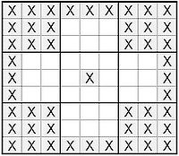
Constraints of Clue Geometry
It has been postulated that no proper sudoku can have clues limited to the range of positions in the pattern below.One such example is the following with 22 clues:
Automorphic Sudokus
Automorphic sudokus are sudoku puzzles which solve to an automorphic grid. A grid is automorphic if it can be transformed in a way that leads back to the original grid, when that same transformation would not otherwise lead back to the original grid. An example of a grid which is automorphic would be a grid which can be rotated 180 degrees resulting in a new grid where the new cell values are a permutation of the original grid. An example of an automorphic sudoku which solves to such a grid is below.Notice that if this sudoku is rotated 180 degrees, and the clues relabeled with the permutation (123456789) -> (987654321), it returns to the same sudoku. Expressed another way, this sudoku has the property that every 180 degree rotational pair of clues (a, b) follows the rule (a) + (b) = 10.
Since this sudoku is automorphic, so too its solution grid must be automorphic. Furthermore, every cell which is solved has a symmetrical partner which is solved with the same technique (and the pair would take the form a + b = 10).
In this example the automorphism is easy to identify, but in general automorphism is not always obvious. There are several types of transformations of a sudoku, and therefore automorphism can take several different forms too. Among the population of all sudoku grids, those that are automorphic are rare. They are considered interesting because of their intrinsic mathematical symmetry.
See also
- SudokuSudokuis a logic-based, combinatorial number-placement puzzle. The objective is to fill a 9×9 grid with digits so that each column, each row, and each of the nine 3×3 sub-grids that compose the grid contains all of the digits from 1 to 9...
- main Sudoku article - List of Sudoku terms and jargon
- Dancing LinksDancing LinksIn computer science, Dancing Links, also known as DLX, is the technique suggested by Donald Knuth to efficiently implement his Algorithm X. Algorithm X is a recursive, nondeterministic, depth-first, backtracking algorithm that finds all solutions to the exact cover problem...
- Donald Knuth - Algorithmics of sudokuAlgorithmics of sudokuThe class of Sudoku puzzles consists of a partially completed row-column grid of cells partitioned into N regions or zones each of size N cells, to be filled in using a prescribed set of N distinct symbols , so that each row, column and region contains exactly one of each element of the set...
External links
- Enumerating possible Sudoku grids by Felgenhauer and Jarvis, describes the all-solutions calculation
- V. Elser's difference-map algorithm also solves Sudoku
- Sudoku Puzzle - an Exercise in Constraint Programming and Visual Prolog 7 by Carsten Kehler Holst (in Visual PrologVisual PrologVisual Prolog, also formerly known as PDC Prolog and Turbo Prolog, is a strongly typed object-oriented extension of Prolog. As Turbo Prolog it was marketed by Borland, but it is now developed and marketed by the Danish firm Prolog Development Center that originally developed it...
) - Sudoku Squares and Chromatic Polynomials by Herzberg and Murty, treats Sudoku puzzles as vertex coloringGraph coloringIn graph theory, graph coloring is a special case of graph labeling; it is an assignment of labels traditionally called "colors" to elements of a graph subject to certain constraints. In its simplest form, it is a way of coloring the vertices of a graph such that no two adjacent vertices share the...
problems in graph theoryGraph theoryIn mathematics and computer science, graph theory is the study of graphs, mathematical structures used to model pairwise relations between objects from a certain collection. A "graph" in this context refers to a collection of vertices or 'nodes' and a collection of edges that connect pairs of...
.