Algorithmic inference
Encyclopedia
Algorithmic inference gathers new developments in the statistical inference
methods made feasible by the powerful computing devices widely available to any data analyst. Cornerstones in this field are computational learning theory
, granular computing
, bioinformatics
, and, long ago, structural probability .
The main focus is on the algorithms which compute statistics rooting the study of a random phenomenon, along with the amount of data they must feed on to produce reliable results. This shifts the interest of mathematicians from the study of the distribution laws
to the functional properties of the statistics
, and the interest of computer scientists from the algorithms for processing data to the information
they process.
: is it a physical feature of phenomena to be described through random variables or a way of synthesizing data about a phenomenon? Opting for the latter, Fisher defines a fiducial distribution law of parameters of a given random variable that he deduces from a sample of its specifications. With this law he computes, for instance “the probability that μ (mean of a Gaussian variable – our note) is less than any assigned value, or the probability that it lies between any assigned values, or, in short, its probability distribution, in the light of the sample observed”.
analogous notions, such as Bayes' posterior distribution, Fraser's constructive probability and Neyman's confidence intervals. For half a century, Neyman's confidence intervals won out for all practical purposes, crediting the phenomenological nature of probability. With this perspective, when you deal with a Gaussian variable, its mean μ is fixed by the physical features of the phenomenon you are observing, where the observations are random operators, hence the observed values are specifications of a random sample
. Because of their randomness, you may compute from the sample specific intervals containing the fixed μ with a given probability that you denote confidence.
 and
and 
and a sample drawn from it. Working with statistics
and
is the sample mean, we recognize that
follows a Student's t distribution with parameter (degrees of freedom) m − 1, so that
Gauging T between two quantiles and inverting its expression as a function of you obtain confidence intervals for
  .
.
With the sample specification:

having size m = 10, you compute the statistics and
and  , and obtain a 0.90 confidence interval for
  with extremes (3.03, 5.65).
The classic solution has one benefit and one drawback. The former was appreciated particularly back when people still did computations with sheet and pencil. Per se, the task of computing a Neyman confidence interval for the fixed parameter θ is hard: you don’t know θ, but you look for disposing around it an interval with a possibly very low probability of failing. The analytical solution is allowed for a very limited number of theoretical cases. Vice versa a large variety of instances may be quickly solved in an approximate way via the central limit theorem
in terms of confidence interval around a Gaussian distribution – that's the benefit.
The drawback is that the central limit theorem is applicable when the sample size is sufficiently large. Therefore it is less and less applicable with the sample involved in modern inference instances. The fault is not in the sample size on its own part. Rather, this size is not sufficiently large because of the complexity
of the inference problem.
With the availability of large computing facilities, scientists refocused from isolated parameters inference to complex functions inference, i.e. re sets of highly nested parameters identifying functions. In these cases we speak about learning of functions (in terms for instance of regression
, neuro-fuzzy system
or computational learning
) on the basis of highly informative samples. A first effect of having a complex structure linking data is the reduction of the number of sample degrees of freedom
, i.e. the burning of a part of sample points, so that the effective sample size to be considered in the central limit theorem is too small. Focusing on the sample size ensuring a limited learning error with a given confidence level, the consequence is that the lower bound on this size grows with complexity indices
such as VC dimension
or detail of a class to which the function we want to learn belongs.
 of X with a value
  of the random parameter
  derived from a master equation rooted on a well-behaved statistic s.
{|
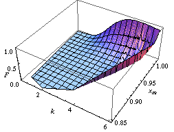
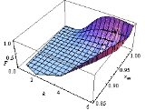
 You may find the distribution law of the Pareto parameters A and K as an implementation example of the population bootstrap method as in the figure on the left.
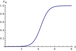
Implementing the twisting argument method, you get the distribution law of the mean M of a Gaussian variable X on the basis of the statistic
  when
when  is known to be equal to
  . Its expression is:

shown in the figure on the right, where is the cumulative distribution function
of a standard normal distribution.
 Computing a confidence interval
for M given its distribution function is straightforward: we need only find two quantiles (for instance and
and  quantiles in case we are interested in a confidence interval of level δ symmetric in the tail's probabilities) as indicated on the left in the diagram showing the behavior of the two bounds for different values of the statistic sm.
The Achilles heel of Fisher's approach lies in the joint distribution of more than one parameter, say mean and variance of a Gaussian distribution. On the contrary, with the last approach (and above-mentioned methods: population bootstrap and twisting argument) we may learn the joint distribution of many parameters. For instance, focusing on the distribution of two or many more parameters, in the figures below we report two confidence regions where the function to be learnt falls with a confidence of 90%. The former concerns the probability with which an extended support vector machine
attributes a binary label 1 to the points of the plane. The two surfaces are drawn on the basis of a set of sample points in turn labelled according to a specific distribution law . The latter concerns the confidence region of the hazard rate of breast cancer recurrence computed from a censored sample .
{|
| |
|  |}
|}
Statistical inference
In statistics, statistical inference is the process of drawing conclusions from data that are subject to random variation, for example, observational errors or sampling variation...
methods made feasible by the powerful computing devices widely available to any data analyst. Cornerstones in this field are computational learning theory
Computational learning theory
In theoretical computer science, computational learning theory is a mathematical field related to the analysis of machine learning algorithms.-Overview:Theoretical results in machine learning mainly deal with a type of...
, granular computing
Granular computing
Granular computing is an emerging computing paradigm of information processing. It concerns the processing of complex information entities called information granules, which arise in the process of data abstraction and derivation of knowledge from information...
, bioinformatics
Bioinformatics
Bioinformatics is the application of computer science and information technology to the field of biology and medicine. Bioinformatics deals with algorithms, databases and information systems, web technologies, artificial intelligence and soft computing, information and computation theory, software...
, and, long ago, structural probability .
The main focus is on the algorithms which compute statistics rooting the study of a random phenomenon, along with the amount of data they must feed on to produce reliable results. This shifts the interest of mathematicians from the study of the distribution laws
Probability distribution
In probability theory, a probability mass, probability density, or probability distribution is a function that describes the probability of a random variable taking certain values....
to the functional properties of the statistics
Statistics
Statistics is the study of the collection, organization, analysis, and interpretation of data. It deals with all aspects of this, including the planning of data collection in terms of the design of surveys and experiments....
, and the interest of computer scientists from the algorithms for processing data to the information
Information
Information in its most restricted technical sense is a message or collection of messages that consists of an ordered sequence of symbols, or it is the meaning that can be interpreted from such a message or collection of messages. Information can be recorded or transmitted. It can be recorded as...
they process.
The Fisher parametric inference problem
Concerning the identification of the parameters of a distribution law, the mature reader may recall lengthy disputes in the mid 20th century about the interpretation of their variability in terms of fiducial distribution , structural probabilities , priors/posteriors , and so on. From an epistemology viewpoint, this entailed a companion dispute as to the nature of probabilityProbability
Probability is ordinarily used to describe an attitude of mind towards some proposition of whose truth we arenot certain. The proposition of interest is usually of the form "Will a specific event occur?" The attitude of mind is of the form "How certain are we that the event will occur?" The...
: is it a physical feature of phenomena to be described through random variables or a way of synthesizing data about a phenomenon? Opting for the latter, Fisher defines a fiducial distribution law of parameters of a given random variable that he deduces from a sample of its specifications. With this law he computes, for instance “the probability that μ (mean of a Gaussian variable – our note) is less than any assigned value, or the probability that it lies between any assigned values, or, in short, its probability distribution, in the light of the sample observed”.
The classic solution
Fisher fought hard to defend the difference and superiority of his notion of parameter distribution in comparison toanalogous notions, such as Bayes' posterior distribution, Fraser's constructive probability and Neyman's confidence intervals. For half a century, Neyman's confidence intervals won out for all practical purposes, crediting the phenomenological nature of probability. With this perspective, when you deal with a Gaussian variable, its mean μ is fixed by the physical features of the phenomenon you are observing, where the observations are random operators, hence the observed values are specifications of a random sample
Random sample
In statistics, a sample is a subject chosen from a population for investigation; a random sample is one chosen by a method involving an unpredictable component...
. Because of their randomness, you may compute from the sample specific intervals containing the fixed μ with a given probability that you denote confidence.
Example
Let X be a Gaussian variable with parameters and
and 
and
 a sample drawn from it. Working with statistics
and
is the sample mean, we recognize that
follows a Student's t distribution with parameter (degrees of freedom) m − 1, so that
Gauging T between two quantiles and inverting its expression as a function of
 you obtain confidence intervals for
  .
.With the sample specification:

having size m = 10, you compute the statistics
 and
and  , and obtain a 0.90 confidence interval for
  with extremes (3.03, 5.65).
Inferring functions with the help of a computer
From a modeling perspective the entire dispute looks like a chicken-egg dilemma: either fixed data by first and probability distribution of their properties as a consequence, or fixed properties by first and probability distribution of the observed data as a corollary.The classic solution has one benefit and one drawback. The former was appreciated particularly back when people still did computations with sheet and pencil. Per se, the task of computing a Neyman confidence interval for the fixed parameter θ is hard: you don’t know θ, but you look for disposing around it an interval with a possibly very low probability of failing. The analytical solution is allowed for a very limited number of theoretical cases. Vice versa a large variety of instances may be quickly solved in an approximate way via the central limit theorem
Central limit theorem
In probability theory, the central limit theorem states conditions under which the mean of a sufficiently large number of independent random variables, each with finite mean and variance, will be approximately normally distributed. The central limit theorem has a number of variants. In its common...
in terms of confidence interval around a Gaussian distribution – that's the benefit.
The drawback is that the central limit theorem is applicable when the sample size is sufficiently large. Therefore it is less and less applicable with the sample involved in modern inference instances. The fault is not in the sample size on its own part. Rather, this size is not sufficiently large because of the complexity
Complexity
In general usage, complexity tends to be used to characterize something with many parts in intricate arrangement. The study of these complex linkages is the main goal of complex systems theory. In science there are at this time a number of approaches to characterizing complexity, many of which are...
of the inference problem.
With the availability of large computing facilities, scientists refocused from isolated parameters inference to complex functions inference, i.e. re sets of highly nested parameters identifying functions. In these cases we speak about learning of functions (in terms for instance of regression
Regression analysis
In statistics, regression analysis includes many techniques for modeling and analyzing several variables, when the focus is on the relationship between a dependent variable and one or more independent variables...
, neuro-fuzzy system
Neuro-fuzzy
In the field of artificial intelligence, neuro-fuzzy refers to combinations of artificial neural networks and fuzzy logic. Neuro-fuzzy was proposed by J. S. R. Jang...
or computational learning
Computational learning theory
In theoretical computer science, computational learning theory is a mathematical field related to the analysis of machine learning algorithms.-Overview:Theoretical results in machine learning mainly deal with a type of...
) on the basis of highly informative samples. A first effect of having a complex structure linking data is the reduction of the number of sample degrees of freedom
Degrees of freedom (statistics)
In statistics, the number of degrees of freedom is the number of values in the final calculation of a statistic that are free to vary.Estimates of statistical parameters can be based upon different amounts of information or data. The number of independent pieces of information that go into the...
, i.e. the burning of a part of sample points, so that the effective sample size to be considered in the central limit theorem is too small. Focusing on the sample size ensuring a limited learning error with a given confidence level, the consequence is that the lower bound on this size grows with complexity indices
Complexity index
Besides complexity intended as a difficulty to compute a function , in modern computer science and in statistics another complexity index of a function stands for denoting its information content, in turn affecting the difficulty of learning the function from examples.Complexity indices in this...
such as VC dimension
VC dimension
In statistical learning theory, or sometimes computational learning theory, the VC dimension is a measure of the capacity of a statistical classification algorithm, defined as the cardinality of the largest set of points that the algorithm can shatter...
or detail of a class to which the function we want to learn belongs.
Example
A sample of 1,000 independent bits is enough to ensure an absolute error of at most 0.081 on the estimation of the parameter p of the underlying Bernoulli variable with a confidence of at least 0.99. The same size cannot guarantee a threshold less than 0.088 with the same confidence 0.99 when the error is identified with the probability that a 20-year-old man living in New York does not fit the ranges of height, weight and waistline observed on 1,000 Big Apple inhabitants. The accuracy shortage occurs because both the VC dimension and the detail of the class of parallelepipeds, among which the one observed from the 1,000 inhabitants' ranges falls, are equal to 6.The general inversion problem solving the Fisher question
With insufficiently large samples, the approach: fixed sample – random properties suggests inference procedures in three steps:| 1. | Sampling mechanism. It consists of a pair  , where the seed Z is a random variable without unknown parameters, while the explaining function , where the seed Z is a random variable without unknown parameters, while the explaining function  is a function mapping from samples of Z to samples of the random variable X we are interested in. The parameter vector is a function mapping from samples of Z to samples of the random variable X we are interested in. The parameter vector  is a specification of the random parameter is a specification of the random parameter  . Its components are the parameters of the X distribution law. The Integral Transform Theorem ensures the existence of such a mechanism for each (scalar or vector) X when the seed coincides with the random variable U uniformly . Its components are the parameters of the X distribution law. The Integral Transform Theorem ensures the existence of such a mechanism for each (scalar or vector) X when the seed coincides with the random variable U uniformlyUniform distribution (continuous) In probability theory and statistics, the continuous uniform distribution or rectangular distribution is a family of probability distributions such that for each member of the family, all intervals of the same length on the distribution's support are equally probable. The support is defined by... distributed in  . .
|
||
| 2. | Master equations. The actual connection between the model and the observed data is tossed in terms of a set of relations between statistics on the data and unknown parameters that come as a corollary of the sampling mechanisms. We call these relations master equations. Pivoting around the statistic  , the general form of a master equation is: , the general form of a master equation is: . .With these relations we may inspect the values of the parameters that could have generated a sample with the observed statistic from a particular setting of the seeds representing the seed of the sample. Hence, to the population of sample seeds corresponds a population of parameters. In order to ensure this population clean properties, it is enough to draw randomly the seed values and involve either sufficient statistics or, simply, well-behaved statistic Well-behaved statistic A well-behaved statistic is a term sometimes used in the theory of statistics to describe part of a procedure. This usage is broadly similar to the use of well-behaved in more general mathematics... s w.r.t. the parameters, in the master equations. For example, the statistics  and and  prove to be sufficient for parameters a and k of a Pareto random variable X. Thanks to the (equivalent form of the) sampling mechanism prove to be sufficient for parameters a and k of a Pareto random variable X. Thanks to the (equivalent form of the) sampling mechanism  we may read them as we may read them as  respectively. |
||
| 3. | Parameter population. Having fixed a set of master equations, you may map sample seeds into parameters either numerically through a population bootstrap, or analytically through a twisting argument. Hence from a population of seeds you obtain a population of parameters.
Compatibility denotes parameters of compatible populations, i.e. of populations that could have generated a sample giving rise to the observed statistics. You may formalize this notion as follows: |
Definition
For a random variable and a sample drawn from it a compatible distribution is a distribution having the same sampling mechanism of X with a value
  of the random parameter
  derived from a master equation rooted on a well-behaved statistic s.
{|
Example


Implementing the twisting argument method, you get the distribution law
 of the mean M of a Gaussian variable X on the basis of the statistic
  when
when  is known to be equal to
  . Its expression is:
shown in the figure on the right, where
 is the cumulative distribution function
Cumulative distribution function
In probability theory and statistics, the cumulative distribution function , or just distribution function, describes the probability that a real-valued random variable X with a given probability distribution will be found at a value less than or equal to x. Intuitively, it is the "area so far"...
of a standard normal distribution.

Confidence interval
In statistics, a confidence interval is a particular kind of interval estimate of a population parameter and is used to indicate the reliability of an estimate. It is an observed interval , in principle different from sample to sample, that frequently includes the parameter of interest, if the...
for M given its distribution function is straightforward: we need only find two quantiles (for instance
 and
and  quantiles in case we are interested in a confidence interval of level δ symmetric in the tail's probabilities) as indicated on the left in the diagram showing the behavior of the two bounds for different values of the statistic sm.
The Achilles heel of Fisher's approach lies in the joint distribution of more than one parameter, say mean and variance of a Gaussian distribution. On the contrary, with the last approach (and above-mentioned methods: population bootstrap and twisting argument) we may learn the joint distribution of many parameters. For instance, focusing on the distribution of two or many more parameters, in the figures below we report two confidence regions where the function to be learnt falls with a confidence of 90%. The former concerns the probability with which an extended support vector machine
Support vector machine
A support vector machine is a concept in statistics and computer science for a set of related supervised learning methods that analyze data and recognize patterns, used for classification and regression analysis...
attributes a binary label 1 to the points of the
 plane. The two surfaces are drawn on the basis of a set of sample points in turn labelled according to a specific distribution law . The latter concerns the confidence region of the hazard rate of breast cancer recurrence computed from a censored sample .
{|
|


 for X with seed U reads:

 , compatible with the observed sample by solving the following system of equations:

 and
and  are the observed statistics and
  a set of uniform seeds. Transferring to the parameters the probability (density) affecting the seeds, you obtain the distribution law of the random parameters A and K compatible with the statistics you have observed.