
Marching squares
Encyclopedia
Marching squares is a computer graphics
algorithm
that generates contours for a two-dimensional scalar field
(rectangular array of individual numerical values). A similar method can be used to contour 2D triangle meshes
.
The contours can be of two kinds:
Marching Squares takes a similar approach to the 3D
Marching Cubes
algorithm:
Apply a threshold to the 2D field to make a binary
image containing:
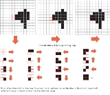
Every 2x2 block of pixels in the binary image forms a contouring cell, so the whole image is represented by a grid of such cells (shown in green in the picture below). Note that this contouring grid is one cell smaller in each direction than the original 2D field.
For each cell in the contouring grid:
data value for the center of the cell to choose between different connections of the interpolated points. Here is another summary of the method showing options for the saddle:
The central value is used to flip the index value before looking-up the cell geometry in the table, i.e. if the index is 0101=5 and the central value is below, then lookup index 10; similarly, if the index is 1010=10 and the central value is below, then lookup index 5.
The index will be ternary
value built from these ternary digits, or trits. We build the index as before, by walking clockwise around the cell, appending each trit to the index, taking the most-significant-trit from the top left corner, and the least-significant-trit from the bottom left corner. There will now be 81 possibilities, rather than 16 for isolines.
Each cell will be filled with 0, 1 or 2 polygonal fragments, each with 3-8 sides.
The action for each cell is based on the category of the ternary index:
The case missing from the 6-sided saddles is for a central value that cannot occur.
There is a valid case omitted from each 7-sided saddle, where the central value is dominated by a single extreme value. The resulting geometric structure would be too complex to fit the simple model of two convex fragments, so it is merged with the case where the central value is within the band. The linear interpolation in such cases will produce a plausible single heptagon.
, which consist of connected triangles with data assigned to the vertices. For example, a scattered set of data points could be connected with a Delaunay triangulation
to allow the data field to be contoured. A triangular cell is always planar, because it is a 2-simplex
(i.e. specified by n+1 vertices in an n-dimensional space). There is always a unique linear interpolant across a triangle and no possibility of an ambiguous saddle.
The analysis for isolines over triangles is especially simple: there are 3 binary digits, so 8 possibilities:
The analysis for isobands over triangles requires 3 ternary trits, so 27 possibilities:
grid, but the spatial coordinates assigned to the vertices can be in 2D, 3D or higher dimensions.
For example, a triangular mesh may represent a 2D data surface embedded in 3D space, where spatial positions of the vertices and interpolated points along a contour will all have 3 coordinates. Note that the case of squares is ambiguous again, because a quadrilateral
embedded in 3-dimensional space is not necessarily planar, so there is a choice of geometrical interpolation scheme to draw the banded surfaces in 3D.
assuming:
A naive implementation of Marching Squares that processes every cell independently will perform every linear interpolation
twice (isoline) or four times (isoband). Similarly, the output will contain 2 copies of the 2D vertices for disjoint lines (isoline) or 4 copies for polygons (isobands). [Under the assumptions that: the grid is large, so that most cells are internal; and a full contiguous set of isobands is being created.]
It is possible to reduce the computational overhead by caching
the results of interpolation. For example, a single-threaded serial version would only need to cache interpolated results for one row of the input grid.
It is also possible to reduce the size of the output by using indexed geometric primitives, i.e. create an array of 2D vertices and specify lines or polygons with short integer offsets into the array.
Computer graphics
Computer graphics are graphics created using computers and, more generally, the representation and manipulation of image data by a computer with help from specialized software and hardware....
algorithm
Algorithm
In mathematics and computer science, an algorithm is an effective method expressed as a finite list of well-defined instructions for calculating a function. Algorithms are used for calculation, data processing, and automated reasoning...
that generates contours for a two-dimensional scalar field
Scalar field
In mathematics and physics, a scalar field associates a scalar value to every point in a space. The scalar may either be a mathematical number, or a physical quantity. Scalar fields are required to be coordinate-independent, meaning that any two observers using the same units will agree on the...
(rectangular array of individual numerical values). A similar method can be used to contour 2D triangle meshes
Triangulated irregular network
A triangulated irregular network is a digital data structure used in a geographic information system for the representation of a surface...
.
The contours can be of two kinds:
- Isolines - lines following a single data level, or isovalue.
- Isobands - filled areas between isolines.
Marching Squares takes a similar approach to the 3D
Three-dimensional space
Three-dimensional space is a geometric 3-parameters model of the physical universe in which we live. These three dimensions are commonly called length, width, and depth , although any three directions can be chosen, provided that they do not lie in the same plane.In physics and mathematics, a...
Marching Cubes
Marching cubes
Marching cubes is a computer graphics algorithm, published in the 1987 SIGGRAPH proceedings by Lorensen and Cline, for extracting a polygonal mesh of an isosurface from a three-dimensional scalar field...
algorithm:
- Process each cell in the grid independently.
- Calculate a cell index using comparisons of the contour level(s) with the data values at the cell corners.
- Use a pre-built lookup tableLookup tableIn computer science, a lookup table is a data structure, usually an array or associative array, often used to replace a runtime computation with a simpler array indexing operation. The savings in terms of processing time can be significant, since retrieving a value from memory is often faster than...
, keyed on the cell index, to describe the output geometry for the cell. - Apply linear interpolationLinear interpolationLinear interpolation is a method of curve fitting using linear polynomials. Lerp is an abbreviation for linear interpolation, which can also be used as a verb .-Linear interpolation between two known points:...
along the boundaries of the cell to calculate the exact contour position.
Basic Algorithm
Here are the steps of the algorithm:Apply a threshold to the 2D field to make a binary
Binary numeral system
The binary numeral system, or base-2 number system, represents numeric values using two symbols, 0 and 1. More specifically, the usual base-2 system is a positional notation with a radix of 2...
image containing:
- 1 where the data value is above the isovalue
- 0 where the data value is below the isovalue
Every 2x2 block of pixels in the binary image forms a contouring cell, so the whole image is represented by a grid of such cells (shown in green in the picture below). Note that this contouring grid is one cell smaller in each direction than the original 2D field.
For each cell in the contouring grid:
- Compose the 4 bitBitA bit is the basic unit of information in computing and telecommunications; it is the amount of information stored by a digital device or other physical system that exists in one of two possible distinct states...
s at the corners of the cell to build a binary index: walk around the cell in a clockwiseClockwiseCircular motion can occur in two possible directions. A clockwise motion is one that proceeds in the same direction as a clock's hands: from the top to the right, then down and then to the left, and back to the top...
direction appending the bitBitA bit is the basic unit of information in computing and telecommunications; it is the amount of information stored by a digital device or other physical system that exists in one of two possible distinct states...
to the index, using bitwise OR and left-shiftLogical shiftIn computer science, a logical shift is a bitwise operation that shifts all the bits of its operand. Unlike an arithmetic shift, a logical shift does not preserve a number's sign bit or distinguish a number's exponent from its mantissa; every bit in the operand is simply moved a given number of bit...
, from most significant bitMost significant bitIn computing, the most significant bit is the bit position in a binary number having the greatest value...
at the top left, to least significant bitLeast significant bitIn computing, the least significant bit is the bit position in a binary integer giving the units value, that is, determining whether the number is even or odd. The lsb is sometimes referred to as the right-most bit, due to the convention in positional notation of writing less significant digits...
at the bottom left. The resulting 4-bit index can have 16 possible values in the range 0-15. - Use the cell index to access a pre-built lookup tableLookup tableIn computer science, a lookup table is a data structure, usually an array or associative array, often used to replace a runtime computation with a simpler array indexing operation. The savings in terms of processing time can be significant, since retrieving a value from memory is often faster than...
with 16 entries listing the edges needed to represent the cell (shown in the lower right part of the picture below). - Apply linear interpolationLinear interpolationLinear interpolation is a method of curve fitting using linear polynomials. Lerp is an abbreviation for linear interpolation, which can also be used as a verb .-Linear interpolation between two known points:...
between the original field data values to find the exact position of the contour line along the edges of the cell.
Disambiguation of Saddle Points
The contour is ambiguous at saddle points. It is possible to resolve the ambiguity by using the averageAverage
In mathematics, an average, or central tendency of a data set is a measure of the "middle" value of the data set. Average is one form of central tendency. Not all central tendencies should be considered definitions of average....
data value for the center of the cell to choose between different connections of the interpolated points. Here is another summary of the method showing options for the saddle:
The central value is used to flip the index value before looking-up the cell geometry in the table, i.e. if the index is 0101=5 and the central value is below, then lookup index 10; similarly, if the index is 1010=10 and the central value is below, then lookup index 5.
Isoband
A similar algorithm can be created for filled contour bands within upper and lower threshold values. To build the index we compare the data values at the cell corners with the two contour threshold values. There are now 3 possibilities:- 0 - corner data value below lower band level
- 1 - corner data value within band interval
- 2 - corner data value above upper level
The index will be ternary
Ternary numeral system
Ternary is the base- numeral system. Analogous to a bit, a ternary digit is a trit . One trit contains \log_2 3 bits of information...
value built from these ternary digits, or trits. We build the index as before, by walking clockwise around the cell, appending each trit to the index, taking the most-significant-trit from the top left corner, and the least-significant-trit from the bottom left corner. There will now be 81 possibilities, rather than 16 for isolines.
Each cell will be filled with 0, 1 or 2 polygonal fragments, each with 3-8 sides.
The action for each cell is based on the category of the ternary index:
- Empty - no fragmemts for index values 0 (0000) or 80 (2222).
- Not Empty - walk around the cell adding corner positions that are within the band and interpolating along relevant edges; use the index to decide how to connect the list of points:
- Slope - build a single polygon fragment with 3-7 sides.
- Saddle - calculate the average value to help disambiguation; then use the index and the central value to build 1 or 2 polygonal fragments with a total of 6, 7 or 8 sides.
The case missing from the 6-sided saddles is for a central value that cannot occur.
There is a valid case omitted from each 7-sided saddle, where the central value is dominated by a single extreme value. The resulting geometric structure would be too complex to fit the simple model of two convex fragments, so it is merged with the case where the central value is within the band. The linear interpolation in such cases will produce a plausible single heptagon.
Meandering Triangles
The same basic algorithm can be applied to triangular meshesTriangulated irregular network
A triangulated irregular network is a digital data structure used in a geographic information system for the representation of a surface...
, which consist of connected triangles with data assigned to the vertices. For example, a scattered set of data points could be connected with a Delaunay triangulation
Delaunay triangulation
In mathematics and computational geometry, a Delaunay triangulation for a set P of points in a plane is a triangulation DT such that no point in P is inside the circumcircle of any triangle in DT. Delaunay triangulations maximize the minimum angle of all the angles of the triangles in the...
to allow the data field to be contoured. A triangular cell is always planar, because it is a 2-simplex
Simplex
In geometry, a simplex is a generalization of the notion of a triangle or tetrahedron to arbitrary dimension. Specifically, an n-simplex is an n-dimensional polytope which is the convex hull of its n + 1 vertices. For example, a 2-simplex is a triangle, a 3-simplex is a tetrahedron,...
(i.e. specified by n+1 vertices in an n-dimensional space). There is always a unique linear interpolant across a triangle and no possibility of an ambiguous saddle.
The analysis for isolines over triangles is especially simple: there are 3 binary digits, so 8 possibilities:
The analysis for isobands over triangles requires 3 ternary trits, so 27 possibilities:
Dimensions and Spaces
The data space for the Marching Squares algorithm is 2D, because the vertices assigned a data value are connected to their neighbors in a 2D topologicalTopology
Topology is a major area of mathematics concerned with properties that are preserved under continuous deformations of objects, such as deformations that involve stretching, but no tearing or gluing...
grid, but the spatial coordinates assigned to the vertices can be in 2D, 3D or higher dimensions.
For example, a triangular mesh may represent a 2D data surface embedded in 3D space, where spatial positions of the vertices and interpolated points along a contour will all have 3 coordinates. Note that the case of squares is ambiguous again, because a quadrilateral
Quadrilateral
In Euclidean plane geometry, a quadrilateral is a polygon with four sides and four vertices or corners. Sometimes, the term quadrangle is used, by analogy with triangle, and sometimes tetragon for consistency with pentagon , hexagon and so on...
embedded in 3-dimensional space is not necessarily planar, so there is a choice of geometrical interpolation scheme to draw the banded surfaces in 3D.
Performance Considerations
The algorithm is embarassingly parallel, because all cells are processed independently. It is easy to write a parallel algorithmParallel algorithm
In computer science, a parallel algorithm or concurrent algorithm, as opposed to a traditional sequential algorithm, is an algorithm which can be executed a piece at a time on many different processing devices, and then put back together again at the end to get the correct result.Some algorithms...
assuming:
- Shared read-only input scalar field.
- Shared append-only geometry output stream.
A naive implementation of Marching Squares that processes every cell independently will perform every linear interpolation
Linear interpolation
Linear interpolation is a method of curve fitting using linear polynomials. Lerp is an abbreviation for linear interpolation, which can also be used as a verb .-Linear interpolation between two known points:...
twice (isoline) or four times (isoband). Similarly, the output will contain 2 copies of the 2D vertices for disjoint lines (isoline) or 4 copies for polygons (isobands). [Under the assumptions that: the grid is large, so that most cells are internal; and a full contiguous set of isobands is being created.]
It is possible to reduce the computational overhead by caching
Cache
In computer engineering, a cache is a component that transparently stores data so that future requests for that data can be served faster. The data that is stored within a cache might be values that have been computed earlier or duplicates of original values that are stored elsewhere...
the results of interpolation. For example, a single-threaded serial version would only need to cache interpolated results for one row of the input grid.
It is also possible to reduce the size of the output by using indexed geometric primitives, i.e. create an array of 2D vertices and specify lines or polygons with short integer offsets into the array.
Links
- Marching Square Matlab algorithm - An easy to understand open-source marching square algorithm.