Kernel principal component analysis
Encyclopedia
Kernel principal component analysis (kernel PCA)
is an extension of principal component analysis (PCA) using techniques of kernel methods
. Using a kernel, the originally linear operations of PCA are done in a reproducing kernel Hilbert space
with a non-linear mapping.
 .
.
It operates by diagonalizing the covariance matrix
,
in other words, it gives an eigendecomposition
of the covariance matrix:
which can be rewritten as .
.
(See also: Covariance matrix as a linear operator)
 dimensions, but can almost always
be linearly separated in dimensions. That is, if we have N points,
  , if we can map them to an N-dimensional space with
 where
where  and
and  is the Kronecker delta.
it is easy to construct a hyperplane
that divides the points into arbitrary clusters. Of course, this creates linearly independent vectors, so there is no covariance on which to perform eigendecomposition explicitly as we would in linear PCA.
Instead, in kernel PCA, a non-trivial, arbitrary function is 'chosen' that is never calculated explicitly, allowing the possibility to use very high dimensional
  's if we never have to actually evaluate the data in that space. Since we generally try to avoid working in the
  -space, which we will call the 'feature space', we can create the N-by-N kernel

which represents the inner product space (see Gramian matrix) of the otherwise intractable feature space. The dual form that arises in the creation of a kernel allows us to mathematically formulate a version of PCA in which we never actually solve the eigenvectors and eigenvalues of the covariance matrix in the -space (see Kernel trick
). The N-elements in each column of K represent the dot product of one point of the transformed data with respect to all the transformed points (N points). Some well-known kernels are shown in the example below.
By imposing the constraint to not work in the feature space, the kernel-formulation of PCA is restricted in that it computes not the principal components themselves, but the projections of our data onto those components. To evaluate the projection from a point in the feature space onto the kth principal component
  (where exponent k means the component k, not powers of k)

We note that denotes dot product, which is simply the elements of the kernel
  . It seems all thats left is to calculate and normalize the
  , which can be done by solving the eigenvector equation

where N is the number of data points in the set, and lambda and a are the eigenvalues and eigenvectors of K. Then to normalize the eigenvectors 's, we require that

Care must be taken regarding the fact that, whether or not has zero-mean in its original space, it is not guaranteed to be centered in the feature space (which we never compute explicitly). Since centered data is required to perform an effective principal component analysis, we 'centralize' K to become

where denotes a N-by-N matrix for which each element takes value
  . We use
  to perform the kernel PCA algorithm described above.
One caveat of kernel PCA should be illustrated here. In linear PCA, we can calculate an 'efficient' number of eigenvalues and perform dimensionality reduction of our data by representing the original data as an approximation, projected onto their eigenvectors. However we can't calculate those eigenvectors with Kernel PCA.
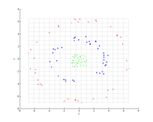
 Consider three concentric clouds of points (shown); we wish to use kernel PCA to identify these groups. The color of the points is not part of the algorithm, but only there to show how the data groups together before and after the transformation.
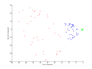
First, consider the kernel
Applying this to kernel PCA yields the next image.
 Now consider a Gaussian kernel:
That is, this kernel is a measure of closeness–1 when the points coincide with a limit of 0 at infinity.
 Note in particular that the first principal component is enough to distinguish the three different groups, which is impossible using only linear PCA, because linear PCA operates only in the given (in this case two-dimensional) space, in which these concentric point clouds are not separable.
is an extension of principal component analysis (PCA) using techniques of kernel methods
Kernel methods
In computer science, kernel methods are a class of algorithms for pattern analysis, whose best known elementis the support vector machine...
. Using a kernel, the originally linear operations of PCA are done in a reproducing kernel Hilbert space
Reproducing kernel Hilbert space
In functional analysis , a reproducing kernel Hilbert space is a Hilbert space of functions in which pointwise evaluation is a continuous linear functional. Equivalently, they are spaces that can be defined by reproducing kernels...
with a non-linear mapping.
Linear PCA
Recall that conventional PCA operates on zero-centered data; that is, .
.It operates by diagonalizing the covariance matrix
Covariance matrix
In probability theory and statistics, a covariance matrix is a matrix whose element in the i, j position is the covariance between the i th and j th elements of a random vector...
,

in other words, it gives an eigendecomposition
Eigendecomposition of a matrix
In the mathematical discipline of linear algebra, eigendecomposition or sometimes spectral decomposition is the factorization of a matrix into a canonical form, whereby the matrix is represented in terms of its eigenvalues and eigenvectors...
of the covariance matrix:

which can be rewritten as
 .
.(See also: Covariance matrix as a linear operator)
Introduction of the Kernel to PCA
To understand the utility of kernel PCA, particularly for clustering, observe that, while N points cannot in general be linearly separated in dimensions, but can almost always
Almost Always
"Almost Always" is a popular song. It was recorded by Joni James in 1953. The recording was released by MGM as catalog number 11470. The song was only on the Billboard magazine charts for one week, reaching #18 on May 9, 1953. The flip side was "Is It Any Wonder?"...
be linearly separated in
 dimensions. That is, if we have N points,
  , if we can map them to an N-dimensional space with
 where
where  and
and  is the Kronecker delta.
it is easy to construct a hyperplane
Hyperplane
A hyperplane is a concept in geometry. It is a generalization of the plane into a different number of dimensions.A hyperplane of an n-dimensional space is a flat subset with dimension n − 1...
that divides the points into arbitrary clusters. Of course, this
 creates linearly independent vectors, so there is no covariance on which to perform eigendecomposition explicitly as we would in linear PCA.
Instead, in kernel PCA, a non-trivial, arbitrary
 function is 'chosen' that is never calculated explicitly, allowing the possibility to use very high dimensional
  's if we never have to actually evaluate the data in that space. Since we generally try to avoid working in the
  -space, which we will call the 'feature space', we can create the N-by-N kernel
which represents the inner product space (see Gramian matrix) of the otherwise intractable feature space. The dual form that arises in the creation of a kernel allows us to mathematically formulate a version of PCA in which we never actually solve the eigenvectors and eigenvalues of the covariance matrix in the
 -space (see Kernel trick
Kernel trick
For machine learning algorithms, the kernel trick is a way of mapping observations from a general set S into an inner product space V , without ever having to compute the mapping explicitly, in the hope that the observations will gain meaningful linear structure in V...
). The N-elements in each column of K represent the dot product of one point of the transformed data with respect to all the transformed points (N points). Some well-known kernels are shown in the example below.
By imposing the constraint to not work in the feature space, the kernel-formulation of PCA is restricted in that it computes not the principal components themselves, but the projections of our data onto those components. To evaluate the projection from a point in the feature space
 onto the kth principal component
  (where exponent k means the component k, not powers of k)
We note that
 denotes dot product, which is simply the elements of the kernel
  . It seems all thats left is to calculate and normalize the
  , which can be done by solving the eigenvector equation
where N is the number of data points in the set, and lambda and a are the eigenvalues and eigenvectors of K. Then to normalize the eigenvectors
 's, we require that
Care must be taken regarding the fact that, whether or not
 has zero-mean in its original space, it is not guaranteed to be centered in the feature space (which we never compute explicitly). Since centered data is required to perform an effective principal component analysis, we 'centralize' K to become

where
 denotes a N-by-N matrix for which each element takes value
  . We use
  to perform the kernel PCA algorithm described above.
One caveat of kernel PCA should be illustrated here. In linear PCA, we can calculate an 'efficient' number of eigenvalues and perform dimensionality reduction of our data by representing the original data as an approximation, projected onto their eigenvectors. However we can't calculate those eigenvectors with Kernel PCA.
Large Datasets
In practice, a large data set leads to a large K, and storing K may become a problem. One way to deal with this is to perform clustering on your large dataset, and populate the kernel with the means of those clusters. Since even this method may yield a relatively large K, it is common to compute only the top P eigenvalues and eigenvectors of K.Example

First, consider the kernel
Applying this to kernel PCA yields the next image.

That is, this kernel is a measure of closeness–1 when the points coincide with a limit of 0 at infinity.

Applications
Kernel PCA has been demonstrated to be useful for novelty detection and image de-noising.See also
- Spectral clustering
- Kernel trickKernel trickFor machine learning algorithms, the kernel trick is a way of mapping observations from a general set S into an inner product space V , without ever having to compute the mapping explicitly, in the hope that the observations will gain meaningful linear structure in V...
- Nonlinear dimensionality reductionNonlinear dimensionality reductionHigh-dimensional data, meaning data that requires more than two or three dimensions to represent, can be difficult to interpret. One approach to simplification is to assume that the data of interest lies on an embedded non-linear manifold within the higher-dimensional space...
- Cluster analysis


