Fractional Brownian motion
Encyclopedia
In probability theory
, a normalized fractional Brownian motion (fBm), also called a fractal Brownian motion, is a continuous-time Gaussian process
BH(t) on [0, T], which starts at zero, has expectation zero for all t in [0, T], and has the following covariance function
:

where H is a real number in (0, 1), called the Hurst index
or Hurst parameter associated with the fractional Brownian motion. It was introduced by .
The value of H determines what kind of process the fBm is:
The increment process, X(t) = BH(t+1) − BH(t), is known as fractional Gaussian noise.

where integration is with respect to the white noise
measure dB(s). This integral turns out to be ill-suited to applications of fractional Brownian motion because of its over-emphasis of the origin .
The idea instead is to use a different fractional integral of white noise to define the process: the Weyl integral
for t > 0 (and similarly for t < 0).
, since in terms of probability distribution
s:
Fractional Brownian motion is the only self-similar Gaussian process
.
trajectories are Hölder continuous
of any order strictly less than H: for each such trajectory, there exists a constant c such that
for every ε > 0.
and box dimension of 2−H.
with respect to fractional Brownian motion, usually called "fractional stochastic integrals". In general though, unlike integrals with respect to regular Brownian motion, fractional stochastic integrals are not Semimartingale
s.
Two realisations are shown below, each showing 1000 points of an fBm, the first with Hurst parameter 0.95 and the second with Hurst parameter 0.55.
 .
.
In order to compute , we can use for instance the Cholesky decomposition method
. An alternative method uses the eigenvalues of :
:
Note that this makes sense because .
.
Note that since the eigenvectors are linearly independent, the matrix is inversible.
where B is a standard Brownian motion and
Where is the Euler hypergeometric integral.
Say we want simulate an fBm at points .
.
The integral may be efficiently computed by Gaussian quadrature
. Hypergeometric functions are part of the GNU scientific library
.
Probability theory
Probability theory is the branch of mathematics concerned with analysis of random phenomena. The central objects of probability theory are random variables, stochastic processes, and events: mathematical abstractions of non-deterministic events or measured quantities that may either be single...
, a normalized fractional Brownian motion (fBm), also called a fractal Brownian motion, is a continuous-time Gaussian process
Gaussian process
In probability theory and statistics, a Gaussian process is a stochastic process whose realisations consist of random values associated with every point in a range of times such that each such random variable has a normal distribution...
BH(t) on [0, T], which starts at zero, has expectation zero for all t in [0, T], and has the following covariance function
Covariance function
In probability theory and statistics, covariance is a measure of how much two variables change together and the covariance function describes the variance of a random variable process or field...
:

where H is a real number in (0, 1), called the Hurst index
Hurst exponent
The Hurst exponent is used as a measure of the long term memory of time series. It relates to the autocorrelations of the time series and the rate at which these decrease as the lag between pairs of values increases....
or Hurst parameter associated with the fractional Brownian motion. It was introduced by .
The value of H determines what kind of process the fBm is:
- if H = 1/2 then the process is in fact a Brownian motionBrownian motionBrownian motion or pedesis is the presumably random drifting of particles suspended in a fluid or the mathematical model used to describe such random movements, which is often called a particle theory.The mathematical model of Brownian motion has several real-world applications...
or Wiener processWiener processIn mathematics, the Wiener process is a continuous-time stochastic process named in honor of Norbert Wiener. It is often called standard Brownian motion, after Robert Brown...
; - if H > 1/2 then the increments of the process are positively correlatedCorrelationIn statistics, dependence refers to any statistical relationship between two random variables or two sets of data. Correlation refers to any of a broad class of statistical relationships involving dependence....
; - if H < 1/2 then the increments of the process are negatively correlated.
The increment process, X(t) = BH(t+1) − BH(t), is known as fractional Gaussian noise.
Background and definition
Prior to the introduction of the fractional Brownian motion, used the Riemann–Liouville fractional integral to define the process
where integration is with respect to the white noise
White noise
White noise is a random signal with a flat power spectral density. In other words, the signal contains equal power within a fixed bandwidth at any center frequency...
measure dB(s). This integral turns out to be ill-suited to applications of fractional Brownian motion because of its over-emphasis of the origin .
The idea instead is to use a different fractional integral of white noise to define the process: the Weyl integral

for t > 0 (and similarly for t < 0).
Self-similarity
The process is self-similarSelf-similarity
In mathematics, a self-similar object is exactly or approximately similar to a part of itself . Many objects in the real world, such as coastlines, are statistically self-similar: parts of them show the same statistical properties at many scales...
, since in terms of probability distribution
Probability distribution
In probability theory, a probability mass, probability density, or probability distribution is a function that describes the probability of a random variable taking certain values....
s:
Fractional Brownian motion is the only self-similar Gaussian process
Gaussian process
In probability theory and statistics, a Gaussian process is a stochastic process whose realisations consist of random values associated with every point in a range of times such that each such random variable has a normal distribution...
.
Stationary increments
It has stationary increments:Long-range dependence
For H > ½ the process exhibits long-range dependence,Regularity
Sample-paths are almost nowhere differentiable. However, almost-allAlmost surely
In probability theory, one says that an event happens almost surely if it happens with probability one. The concept is analogous to the concept of "almost everywhere" in measure theory...
trajectories are Hölder continuous
Hölder condition
In mathematics, a real or complex-valued function ƒ on d-dimensional Euclidean space satisfies a Hölder condition, or is Hölder continuous, when there are nonnegative real constants C, \alpha , such that...
of any order strictly less than H: for each such trajectory, there exists a constant c such that
for every ε > 0.
Dimension
With probability 1, the graph of BH(t) has both Hausdorff dimensionHausdorff dimension
thumb|450px|Estimating the Hausdorff dimension of the coast of Great BritainIn mathematics, the Hausdorff dimension is an extended non-negative real number associated with any metric space. The Hausdorff dimension generalizes the notion of the dimension of a real vector space...
and box dimension of 2−H.
Integration
As for regular Brownian motion, one can define stochastic integralsIto calculus
Itō calculus, named after Kiyoshi Itō, extends the methods of calculus to stochastic processes such as Brownian motion . It has important applications in mathematical finance and stochastic differential equations....
with respect to fractional Brownian motion, usually called "fractional stochastic integrals". In general though, unlike integrals with respect to regular Brownian motion, fractional stochastic integrals are not Semimartingale
Semimartingale
In probability theory, a real valued process X is called a semimartingale if it can be decomposed as the sum of a local martingale and an adapted finite-variation process....
s.
Sample paths
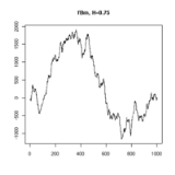
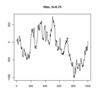
Practical computer realisations of an fBm can be generated, although they are only a finite approximation. The sample paths chosen can be thought of as showing discrete sampled points on an fBm process. Three realisations are shown below, each with 1000 points of an fBm with Hurst parameter 0.75.  |
 |
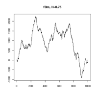 |
| H = 0.75 realisation 1 | H = 0.75 realisation 2 | H = 0.75 realisation 3 |
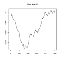
Two realisations are shown below, each showing 1000 points of an fBm, the first with Hurst parameter 0.95 and the second with Hurst parameter 0.55.
 |
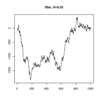 |
| H = 0.95 | H = 0.55 |
Method 1 of simulation
One can simulate sample-paths of an fBm as any Gaussian process of known covariance. Suppose we want to simulate the values of the fBM at times .
.- Form the matrix
 where
where  .
.
- Compute
 the square root matrix of
  , i.e.
  . Loosely speaking,
  is the "standard deviation" matrix associated to the variance-covariance matrix
  .
.
- Construct a vector
 of n numbers drawn according a standard Gaussian distribution,
- If we define
 then
then  yields a sample path of an fBm.
In order to compute
 , we can use for instance the Cholesky decomposition method
Cholesky decomposition
In linear algebra, the Cholesky decomposition or Cholesky triangle is a decomposition of a Hermitian, positive-definite matrix into the product of a lower triangular matrix and its conjugate transpose. It was discovered by André-Louis Cholesky for real matrices...
. An alternative method uses the eigenvalues of
 :
:- Since
 is symmetric, positive-definitePositive-definite matrixIn linear algebra, a positive-definite matrix is a matrix that in many ways is analogous to a positive real number. The notion is closely related to a positive-definite symmetric bilinear form ....
matrix, it follows that all eigenvalues of
of  satisfy
  , (
, ( ).
).
- Let
 be the diagonal matrix of the eigenvalues, i.e.
  where
where  is the Kronecker delta. We define
  as the diagonal matrix with entries
  , i.e.
  .
.
Note that this makes sense because
 .
.- Let
 an eigenvector associated to the eigenvalue
  . Define
  as the matrix whose
  -th column is the eigenvector
  .
.
Note that since the eigenvectors are linearly independent, the matrix
 is inversible.
- It follows then that
 because
  .
.
Method 2 of simulation
It is also known thatwhere B is a standard Brownian motion and
Where
 is the Euler hypergeometric integral.
Say we want simulate an fBm at points
 .
.- Construct a vector of n numbers drawn according a standard Gaussian distribution.
- Multiply it component-wise by √(T/n) to obtain the increments of a Brownian motion on [0, T]. Denote this vector by
 .
.
- For each
 , compute
The integral may be efficiently computed by Gaussian quadrature
Gaussian quadrature
In numerical analysis, a quadrature rule is an approximation of the definite integral of a function, usually stated as a weighted sum of function values at specified points within the domain of integration....
. Hypergeometric functions are part of the GNU scientific library
GNU Scientific Library
In computing, the GNU Scientific Library is a software library written in the C programming language for numerical calculations in applied mathematics and science...
.
See also
- Brownian surfaceBrownian surfaceA Brownian surface is a fractal surface generated via a fractal elevation function.For instance, in the three-dimensional case, where two variables X and Y are given as coordinates, the elevation function between any two points and can be set to have a mean or expected value that increases as the...
- Autoregressive fractionally integrated moving averageAutoregressive fractionally integrated moving averageIn statistics, autoregressive fractionally integrated moving average models are time series models that generalize ARIMA models by allowing non-integer values of the differencing parameter and are useful in modeling time series with long memory...
- Multifractal: The generalized framework of fractional Brownian motions.
- Pink noisePink noisePink noise or 1/ƒ noise is a signal or process with a frequency spectrum such that the power spectral density is inversely proportional to the frequency. In pink noise, each octave carries an equal amount of noise power...


