
Finite deformation tensors
Encyclopedia
In continuum mechanics
, the finite strain theory—also called large strain theory, or large deformation theory—deals with deformations
in which both rotations and strains are arbitrarily large, i.e. invalidates the assumptions inherent in infinitesimal strain theory. In this case, the undeformed and deformed configurations of the continuum
are significantly different and a clear distinction has to be made between them. This is commonly the case with elastomer
s, plastically-deforming
materials and other fluid
s and biological soft tissue
.
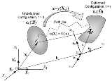
. The displacement of a body has two components: a rigid-body displacement and a deformation. A rigid-body displacement consists of a simultaneous translation and rotation of the body without changing its shape or size. Deformation implies the change in shape and/or size of the body from an initial or undeformed configuration to a current or deformed configuration
  (Figure 1).
If after a displacement of the continuum there is a relative displacement between particles, a deformation has occurred. On the other hand, if after displacement of the continuum the relative displacement between particles in the current configuration is zero i.e. the distance between particles remains unchanged, then there is no deformation and a rigid-body displacement is said to have occurred.
The vector joining the positions of a particle in the undeformed configuration and deformed configuration is called the displacement vector
 in the Lagrangian description, or
  in the Eulerian description, where
  and
and  are respectively Euler-Almansi strain tensor and Green-Lagrange strain tensor.
A displacement field is a vector field of all displacement vectors for all particles in the body, which relates the deformed configuration with the undeformed configuration. It is convenient to do the analysis of deformation or motion of a continuum body in terms of the displacement field. In general, the displacement field is expressed in terms of the material coordinates as

or in terms of the spatial coordinates as

where are the direction cosines between the material and spatial coordinate systems with unit vectors
  and
and  , respectively. Thus

and the relationship between and
and  is then given by

Knowing that
then
It is common to superimpose the coordinate systems for the undeformed and deformed configurations, which results in , and the direction cosines become Kronecker deltas, i.e.

Thus, we have

or in terms of the spatial coordinates as

 . Thus we have,

where is the deformation gradient tensor.
Similarly, the partial differentiation of the displacement vector with respect to the spatial coordinates yields the spatial displacement gradient tensor . Thus we have,

 Consider a particle or material point
 with position vector
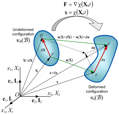
  in the undeformed configuration (Figure 2). After a displacement of the body, the new position of the particle indicated by
  in the new configuration is given by the vector position
  . The coordinate systems for the undeformed and deformed configuration can be superimposed for convenience.
Consider now a material point neighboring
  , with position vector
  . In the deformed configuration this particle has a new position
  given by the position vector
  . Assuming that the line segments
  and
and  joining the particles
  and
and  in both the undeformed and deformed configuration, respectively, to be very small, then we can express them as
  and
and  . Thus from Figure 2 we have

where is the relative displacement vector, which represents the relative displacement of
  with respect to
  in the deformed configuration.
For an infinitesimal element , and assuming continuity on the displacement field, it is possible to use a Taylor series expansion around point
  , neglecting higher-order terms, to approximate the components of the relative displacement vector for the neighboring particle
  as
as

Thus, the previous equation can be written as

The material deformation gradient tensor is a second-order tensor that represents the gradient of the mapping function or functional relation
  , which describes the motion of a continuum
. The material deformation gradient tensor characterizes the local deformation at a material point with position vector , i.e. deformation at neighbouring points, by transforming (linear transformation
) a material line element emanating from that point from the reference configuration to the current or deformed configuration, assuming continuity in the mapping function , i.e. differentiable function
of and time
  , which implies that crack
s and voids do not open or close during the deformation. Thus we have,

The deformation gradient tensor is related to both the reference and current configuration, as seen by the unit vectors
  and
and  , therefore it is a two-point tensor.
Due to the assumption of continuity of ,
,  has the inverse
  , where
  is the spatial deformation gradient tensor. Then, by the implicit function theorem
(Lubliner), the Jacobian determinant must be nonsingular, i.e.

where is an area of a region in the deformed configuration,
  is the same area in the reference configuration, and
  is the outward normal to the area element in the current configuration while
  is the outward normal in the reference configuration,
  is the deformation gradient, and
  .
.
 The deformation gradient
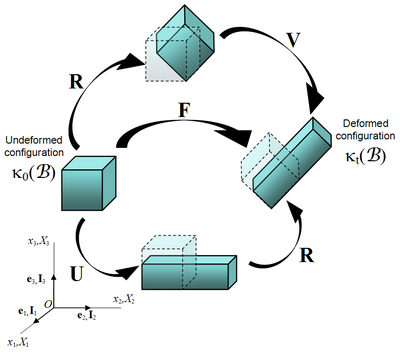
  , like any second-order tensor, can be decomposed, using the polar decomposition theorem, into a product of two second-order tensors (Truesdell and Noll, 1965): an orthogonal tensor and a positive definite symmetric tensor, i.e.

where the tensor is a proper orthogonal tensor, i.e.
  and
and  , representing a rotation; the tensor
  is the right stretch tensor; and
  the left stretch tensor. The terms right and left means that they are to the right and left of the rotation tensor
  , respectively.
  and
and  are both positive definite
, i.e. and
and  , and symmetric tensors, i.e.
  and
and  , of second order.
This decomposition implies that the deformation of a line element in the undeformed configuration onto
  in the deformed configuration, i.e.
  , may be obtained either by first stretching the element by
  , i.e.
  , followed by a rotation
  , i.e.
  ; or equivalently, by applying a rigid rotation
  first, i.e.
  , followed later by a stretching
  , i.e.
  (See Figure 3).
It can be shown that,

so that and
and  have the same eigenvalues or principal stretches, but different eigenvectors or principal directions
  and
and  , respectively. The principal directions are related by

This polar decomposition is unique as is non-symmetric.
Since a pure rotation should not induce any stresses in a deformable body, it is often convenient to use rotation-independent measures of deformation in continuum mechanics
. As a rotation followed by its inverse rotation leads to no change ( ) we can exclude the rotation by multiplying
  by its transpose
.
introduced a deformation tensor known as the right Cauchy-Green deformation tensor or Green's deformation tensor, defined as:

Physically, the Cauchy-Green tensor gives us the square of local change in distances due to deformation, i.e.
Invariants of are often used in the expressions for strain energy density function
s. The most commonly used invariants
are
The IUPAC recommends that the inverse of the right Cauchy-Green deformation tensor (called the Cauchy tensor in that document), i. e., , be called the Finger tensor. However, that nomenclature is not universally accepted in applied mechanics.


The left Cauchy-Green deformation tensor is often called the Finger deformation tensor, named after Josef Finger
(1894).
Invariants of are also used in the expressions for strain energy density function
s. The conventional invariants are defined as
where is the determinant of the deformation gradient.
For nearly incompressible materials, a slightly different set of invariants is used:
introduced a deformation tensor defined as the inverse of the left Cauchy-Green deformation tensor, . This tensor has also been called the Piola tensor and the Finger tensor in the rheology and fluid dynamics literature.

 , the spectral decompositions of
  and
and  is given by

Furthermore,


Observe that
Therefore the uniqueness of the spectral decomposition also implies that . The left stretch (
 ) is also called the spatial stretch tensor while the right stretch (
 ) is called the material stretch tensor.
The effect of acting on
  is to stretch the vector by
  and to rotate it to the new orientation
  , i.e.,
In a similar vein,
of the stretch with respect to the right Cauchy-Green deformation tensor are used to derive the stress-strain relations of many solids, particularly hyperelastic material
s. These derivatives are
and follow from the observations that
 be a Cartesian coordinate system defined on the undeformed body and let
  be another system defined on the deformed body. Let a curve
  in the undeformed body be parametrized using
  . Its image in the deformed body is
  .
.
The undeformed length of the curve is given by
After deformation, the length becomes
Note that the right Cauchy-Green deformation tensor is defined as
Hence,
which indicates that changes in length are characterized by .
.

or as a function of the displacement gradient tensor
or
The Green-Lagrangian strain tensor is a measure of how much differs from
  . It can be shown that this tensor is a special case of a general formula for Lagrangian strain tensors (Hill 1968):

For different values of we have:

The Eulerian-Almansi finite strain tensor, referenced to the deformed configuration, i.e. Eulerian description, is defined as

or as a function of the displacement gradients we have
The stretch ratio for the differential element (Figure) in the direction of the unit vector
  at the material point
  , in the undeformed configuration, is defined as

where is the deformed magnitude of the differential element
  .
.
Similarly, the stretch ratio for the differential element (Figure), in the direction of the unit vector
  at the material point
  , in the deformed configuration, is defined as

The normal strain in any direction
  can be expressed as a function of the stretch ratio,

This equation implies that the normal strain is zero, i.e. no deformation, when the stretch is equal to unity. Some materials, such as elastometers can sustain stretch ratios of 3 or 4 before they fail, whereas traditional engineering materials, such as concrete or steel, fail at much lower stretch ratios, perhaps of the order of 1.001 (reference?)
 of the Lagrangian finite strain tensor are related to the normal strain, e.g.

where is the normal strain or engineering strain in the direction
  .
.
The off-diagonal components of the Lagrangian finite strain tensor are related to shear strain, e.g.

where is the change in the angle between two line elements that were originally perpendicular with directions
  and
and  , respectively.
Under certain circumstances, i.e. small displacements and small displacement rates, the components of the Lagrangian finite strain tensor may be approximated by the components of the infinitesimal strain tensor
is useful for many problems in continuum mechanics such as nonlinear shell theories and large plastic deformations. Let be a given deformation where the space is characterized by the coordinates
  . The tangent vector to the coordinate curve
  at
at  is given by
The three tangent vectors at form a basis. These vectors are related the reciprocal basis vectors by
Let us define a field
The Christoffel symbols of the first kind
can be expressed as
To see how the Christoffel symbols are related to the Right Cauchy-Green deformation tensor let us define two sets of bases
in curvilinear coordinates, the deformation gradient can be written as

If we express in terms of components with respect to the basis {
 } we have
Therefore
and the Christoffel symbol of the first kind may be written in the following form.
 to
to  and let us assume that there exist two positive definite, symmetric second-order tensor fields
  and
and  that satisfy
Then,
Noting that
and we have
Define
Hence
Define
Then
Define the Christoffel symbols of the second kind as
Then
Therefore
The invertibility of the mapping implies that
We can also formulate a similar result in terms of derivatives with respect to . Therefore
 field over a simply connected body are
 field over a simply connected body are
We can show these are the mixed components of the Riemann-Christoffel curvature tensor. Therefore the necessary conditions for -compatibility are that the Riemann-Christoffel curvature of the deformation is zero.
 fields have been found by Janet Blume.
Continuum mechanics
Continuum mechanics is a branch of mechanics that deals with the analysis of the kinematics and the mechanical behavior of materials modelled as a continuous mass rather than as discrete particles...
, the finite strain theory—also called large strain theory, or large deformation theory—deals with deformations
Deformation (mechanics)
Deformation in continuum mechanics is the transformation of a body from a reference configuration to a current configuration. A configuration is a set containing the positions of all particles of the body...
in which both rotations and strains are arbitrarily large, i.e. invalidates the assumptions inherent in infinitesimal strain theory. In this case, the undeformed and deformed configurations of the continuum
Continuum mechanics
Continuum mechanics is a branch of mechanics that deals with the analysis of the kinematics and the mechanical behavior of materials modelled as a continuous mass rather than as discrete particles...
are significantly different and a clear distinction has to be made between them. This is commonly the case with elastomer
Elastomer
An elastomer is a polymer with the property of viscoelasticity , generally having notably low Young's modulus and high yield strain compared with other materials. The term, which is derived from elastic polymer, is often used interchangeably with the term rubber, although the latter is preferred...
s, plastically-deforming
Plasticity (physics)
In physics and materials science, plasticity describes the deformation of a material undergoing non-reversible changes of shape in response to applied forces. For example, a solid piece of metal being bent or pounded into a new shape displays plasticity as permanent changes occur within the...
materials and other fluid
Fluid
In physics, a fluid is a substance that continually deforms under an applied shear stress. Fluids are a subset of the phases of matter and include liquids, gases, plasmas and, to some extent, plastic solids....
s and biological soft tissue
Soft tissue
In anatomy, the term soft tissue refers to tissues that connect, support, or surround other structures and organs of the body, not being bone. Soft tissue includes tendons, ligaments, fascia, skin, fibrous tissues, fat, and synovial membranes , and muscles, nerves and blood vessels .It is sometimes...
.
Displacement
A change in the configuration of a continuum body results in a displacementDisplacement field (mechanics)
A displacement field is an assignment of displacement vectors for all points in a region or body that is displaced from one state to another. A displacement vector specifies the position of a point or a particle in reference to an origin or to a previous position...
. The displacement of a body has two components: a rigid-body displacement and a deformation. A rigid-body displacement consists of a simultaneous translation and rotation of the body without changing its shape or size. Deformation implies the change in shape and/or size of the body from an initial or undeformed configuration
to a current or deformed configuration (Figure 1).If after a displacement of the continuum there is a relative displacement between particles, a deformation has occurred. On the other hand, if after displacement of the continuum the relative displacement between particles in the current configuration is zero i.e. the distance between particles remains unchanged, then there is no deformation and a rigid-body displacement is said to have occurred.
The vector joining the positions of a particle
in the undeformed configuration and deformed configuration is called the displacement vectorDisplacement (vector)
A displacement is the shortest distance from the initial to the final position of a point P. Thus, it is the length of an imaginary straight path, typically distinct from the path actually travelled by P...
in the Lagrangian description, or in the Eulerian description, where and are respectively Euler-Almansi strain tensor and Green-Lagrange strain tensor.A displacement field is a vector field of all displacement vectors for all particles in the body, which relates the deformed configuration with the undeformed configuration. It is convenient to do the analysis of deformation or motion of a continuum body in terms of the displacement field. In general, the displacement field is expressed in terms of the material coordinates as
or in terms of the spatial coordinates as
where
are the direction cosines between the material and spatial coordinate systems with unit vectors and , respectively. Thusand the relationship between
and is then given byKnowing that
then
It is common to superimpose the coordinate systems for the undeformed and deformed configurations, which results in
, and the direction cosines become Kronecker deltas, i.e.Thus, we have
or in terms of the spatial coordinates as
Displacement gradient tensor
The partial differentiation of the displacement vector with respect to the material coordinates yields the material displacement gradient tensor. Thus we have,where
is the deformation gradient tensor.Similarly, the partial differentiation of the displacement vector with respect to the spatial coordinates yields the spatial displacement gradient tensor
. Thus we have,Deformation gradient tensor
Continuum mechanics
Continuum mechanics is a branch of mechanics that deals with the analysis of the kinematics and the mechanical behavior of materials modelled as a continuous mass rather than as discrete particles...
with position vector in the undeformed configuration (Figure 2). After a displacement of the body, the new position of the particle indicated by in the new configuration is given by the vector position . The coordinate systems for the undeformed and deformed configuration can be superimposed for convenience.Consider now a material point
neighboring , with position vector . In the deformed configuration this particle has a new position given by the position vector . Assuming that the line segments and joining the particles and in both the undeformed and deformed configuration, respectively, to be very small, then we can express them as and . Thus from Figure 2 we havewhere
is the relative displacement vector, which represents the relative displacement of with respect to in the deformed configuration.For an infinitesimal element
, and assuming continuity on the displacement field, it is possible to use a Taylor series expansion around point , neglecting higher-order terms, to approximate the components of the relative displacement vector for the neighboring particle asThus, the previous equation
can be written asThe material deformation gradient tensor
is a second-order tensor that represents the gradient of the mapping function or functional relation , which describes the motion of a continuumContinuum mechanics
Continuum mechanics is a branch of mechanics that deals with the analysis of the kinematics and the mechanical behavior of materials modelled as a continuous mass rather than as discrete particles...
. The material deformation gradient tensor characterizes the local deformation at a material point with position vector
, i.e. deformation at neighbouring points, by transforming (linear transformationLinear transformation
In mathematics, a linear map, linear mapping, linear transformation, or linear operator is a function between two vector spaces that preserves the operations of vector addition and scalar multiplication. As a result, it always maps straight lines to straight lines or 0...
) a material line element emanating from that point from the reference configuration to the current or deformed configuration, assuming continuity in the mapping function
, i.e. differentiable functionDifferentiable function
In calculus , a differentiable function is a function whose derivative exists at each point in its domain. The graph of a differentiable function must have a non-vertical tangent line at each point in its domain...
of
and time , which implies that crackFracture
A fracture is the separation of an object or material into two, or more, pieces under the action of stress.The word fracture is often applied to bones of living creatures , or to crystals or crystalline materials, such as gemstones or metal...
s and voids do not open or close during the deformation. Thus we have,
The deformation gradient tensor
is related to both the reference and current configuration, as seen by the unit vectors and , therefore it is a two-point tensor.Due to the assumption of continuity of
, has the inverse , where is the spatial deformation gradient tensor. Then, by the implicit function theoremImplicit function theorem
In multivariable calculus, the implicit function theorem is a tool which allows relations to be converted to functions. It does this by representing the relation as the graph of a function. There may not be a single function whose graph is the entire relation, but there may be such a function on...
(Lubliner), the Jacobian determinant
must be nonsingular, i.e. Transformation of a surface and volume element
To transform quantities that are defined with respect to areas in a deformed configuration to those relative to areas in a reference configuration, and vice versa, we use the Nanson's relation, expressed aswhere
is an area of a region in the deformed configuration, is the same area in the reference configuration, and is the outward normal to the area element in the current configuration while is the outward normal in the reference configuration, is the deformation gradient, and .| Derivation of Nanson's relation |
|---|
| To see how this formula is derived, we start with the oriented area elements in the reference and current configurations:  The reference and current volumes of an element are  where  . .Therefore,  or,  or,  So we get  or,  |
Polar decomposition of the deformation gradient tensor
, like any second-order tensor, can be decomposed, using the polar decomposition theorem, into a product of two second-order tensors (Truesdell and Noll, 1965): an orthogonal tensor and a positive definite symmetric tensor, i.e.where the tensor
is a proper orthogonal tensor, i.e. and , representing a rotation; the tensor is the right stretch tensor; and the left stretch tensor. The terms right and left means that they are to the right and left of the rotation tensor , respectively. and are both positive definitePositive-definite matrix
In linear algebra, a positive-definite matrix is a matrix that in many ways is analogous to a positive real number. The notion is closely related to a positive-definite symmetric bilinear form ....
, i.e.
and , and symmetric tensors, i.e. and , of second order.This decomposition implies that the deformation of a line element
in the undeformed configuration onto in the deformed configuration, i.e. , may be obtained either by first stretching the element by , i.e. , followed by a rotation , i.e. ; or equivalently, by applying a rigid rotation first, i.e. , followed later by a stretching , i.e. (See Figure 3).It can be shown that,
so that
and have the same eigenvalues or principal stretches, but different eigenvectors or principal directions and , respectively. The principal directions are related byThis polar decomposition is unique as
is non-symmetric.Deformation tensors
Several rotation-independent deformation tensors are used in mechanics. In solid mechanics, the most popular of these are the right and left Cauchy-Green deformation tensors.Since a pure rotation should not induce any stresses in a deformable body, it is often convenient to use rotation-independent measures of deformation in continuum mechanics
Continuum mechanics
Continuum mechanics is a branch of mechanics that deals with the analysis of the kinematics and the mechanical behavior of materials modelled as a continuous mass rather than as discrete particles...
. As a rotation followed by its inverse rotation leads to no change (
) we can exclude the rotation by multiplying by its transposeTranspose
In linear algebra, the transpose of a matrix A is another matrix AT created by any one of the following equivalent actions:...
.
The Right Cauchy-Green deformation tensor
In 1839, George GreenGeorge Green
George Green was a British mathematical physicist who wrote An Essay on the Application of Mathematical Analysis to the Theories of Electricity and Magnetism...
introduced a deformation tensor known as the right Cauchy-Green deformation tensor or Green's deformation tensor, defined as:
Physically, the Cauchy-Green tensor gives us the square of local change in distances due to deformation, i.e.
Invariants of
are often used in the expressions for strain energy density functionStrain energy density function
A strain energy density function or stored energy density function is a scalar valued function that relates the strain energy density of a material to the deformation gradient....
s. The most commonly used invariants
Invariants of tensors
In mathematics, in the fields of multilinear algebra and representation theory, invariants of tensors are coefficients of the characteristic polynomial of the tensor A:\ p:=\det ,...
are
The Finger deformation tensor
WARNING: I do not have access to the IUPAC document, but this section contradicts Truesdell, Ehringen, Malvern, Marsden & Hughes, etc., all of which are leading references in continuum mechanics. Anybody with access to the IUPAC document cited below please verify and clarify. Thanks. -- Re: I (this is another I) have checked this and that is correct. But I am no expert in this matter. Note: none of those 'leading references' was in the commission (approximately 20 titular/contributing members) during the preparation of the report, 1993-1997The IUPAC recommends that the inverse of the right Cauchy-Green deformation tensor (called the Cauchy tensor in that document), i. e.,
, be called the Finger tensor. However, that nomenclature is not universally accepted in applied mechanics.The Left Cauchy-Green or Finger deformation tensor
Reversing the order of multiplication in the formula for the right Green-Cauchy deformation tensor leads to the left Cauchy-Green deformation tensor which is defined as:The left Cauchy-Green deformation tensor is often called the Finger deformation tensor, named after Josef Finger
Josef Finger
Josef Finger was an Austrian physicist and mathematician.- Life :Joseph Finger was born the son of a baker in Pilsen. He attended high school in Pilsen. He studied mathematics and physics at Charles University in Prague from 1859 to 1862...
(1894).
Invariants of
are also used in the expressions for strain energy density functionStrain energy density function
A strain energy density function or stored energy density function is a scalar valued function that relates the strain energy density of a material to the deformation gradient....
s. The conventional invariants are defined as
where
is the determinant of the deformation gradient.For nearly incompressible materials, a slightly different set of invariants is used:
The Cauchy deformation tensor
Earlier in 1828 , Augustin Louis CauchyAugustin Louis Cauchy
Baron Augustin-Louis Cauchy was a French mathematician who was an early pioneer of analysis. He started the project of formulating and proving the theorems of infinitesimal calculus in a rigorous manner, rejecting the heuristic principle of the generality of algebra exploited by earlier authors...
introduced a deformation tensor defined as the inverse of the left Cauchy-Green deformation tensor,
. This tensor has also been called the Piola tensor and the Finger tensor in the rheology and fluid dynamics literature.Spectral representation
If there are three distinct principal stretches, the spectral decompositions of and is given byFurthermore,
Observe that
Therefore the uniqueness of the spectral decomposition also implies that
. The left stretch () is also called the spatial stretch tensor while the right stretch () is called the material stretch tensor.The effect of
acting on is to stretch the vector by and to rotate it to the new orientation , i.e.,In a similar vein,
| Examples |
|---|
| Uniaxial extension of an incompressible material This is the case where a specimen is stretched in 1-direction with a stretch ratio of  . If the volume remains constant, the contraction in the other two directions is such that . If the volume remains constant, the contraction in the other two directions is such that  or or  . Then: . Then:  Simple shear    Rigid body rotation   |
Derivatives of stretch
DerivativesTensor derivative (continuum mechanics)
The derivatives of scalars, vectors, and second-order tensors with respect to second-order tensors are of considerable use in continuum mechanics. These derivatives are used in the theories of nonlinear elasticity and plasticity, particularly in the design of algorithms for numerical...
of the stretch with respect to the right Cauchy-Green deformation tensor are used to derive the stress-strain relations of many solids, particularly hyperelastic material
Hyperelastic material
A hyperelastic or Green elastic material is a type of constitutive model for ideally elastic material for which the stress-strain relationship derives from a strain energy density function. The hyperelastic material is a special case of a Cauchy elastic material.For many materials, linear elastic...
s. These derivatives are
and follow from the observations that
Physical interpretation of deformation tensors
Let be a Cartesian coordinate system defined on the undeformed body and let be another system defined on the deformed body. Let a curve in the undeformed body be parametrized using . Its image in the deformed body is .The undeformed length of the curve is given by
After deformation, the length becomes
Note that the right Cauchy-Green deformation tensor is defined as
Hence,
which indicates that changes in length are characterized by
.Finite strain tensors
The concept of strain is used to evaluate how much a given displacement differs locally from a rigid body displacement (Ref. Lubliner). One of such strains for large deformations is the Lagrangian finite strain tensor, also called the Green-Lagrangian strain tensor or Green - St-Venant strain tensor, defined asor as a function of the displacement gradient tensor
or
The Green-Lagrangian strain tensor is a measure of how much
differs from . It can be shown that this tensor is a special case of a general formula for Lagrangian strain tensors (Hill 1968):For different values of
we have:The Eulerian-Almansi finite strain tensor, referenced to the deformed configuration, i.e. Eulerian description, is defined as
or as a function of the displacement gradients we have
| Derivation of the Lagrangian and Eulerain finite strain tensors |
|---|
A measure of deformation is the difference between the squares of the differential line element  , in the undeformed configuration, and , in the undeformed configuration, and  , in the deformed configuration (Figure 2). Deformation has occurred if the difference is non zero, otherwise a rigid-body displacement has occurred. Thus we have, , in the deformed configuration (Figure 2). Deformation has occurred if the difference is non zero, otherwise a rigid-body displacement has occurred. Thus we have, In the Lagrangian description, using the material coordinates as the frame of reference, the linear transformation between the differential lines is  Then we have,  where  are the components of the right Cauchy-Green deformation tensor, are the components of the right Cauchy-Green deformation tensor,  . Then, replacing this equation into the first equation we have, . Then, replacing this equation into the first equation we have, or  where  , are the components of a second-order tensor called the Green - St-Venant strain tensor or the Lagrangian finite strain tensor, , are the components of a second-order tensor called the Green - St-Venant strain tensor or the Lagrangian finite strain tensor, In the Eulerian description, using the spatial coordinates as the frame of reference, the linear transformation between the differential lines is  where  are the components of the spatial deformation gradient tensor, are the components of the spatial deformation gradient tensor,  . Thus we have . Thus we have where the second order tensor  is called Cauchy's deformation tensor, is called Cauchy's deformation tensor,  . Then we have, . Then we have, or  where  , are the components of a second-order tensor called the Eulerian-Almansi finite strain tensor, , are the components of a second-order tensor called the Eulerian-Almansi finite strain tensor, Both the Lagrangian and Eulerian finite strain tensors can be conveniently expressed in terms of the displacement gradient tensor. For the Lagrangian strain tensor, first we differentiate the displacement vector  with respect to the material coordinates with respect to the material coordinates  to obtain the material displacement gradient tensor, to obtain the material displacement gradient tensor,   Replacing this equation into the expression for the Lagrangian finite strain tensor we have  or  Similarly, the Eulerian-Almansi finite strain tensor can be expressed as  |
Stretch ratio
The stretch ratio is a measure of the extensional or normal strain of a differential line element, which can be defined at either the undeformed configuration or the deformed configuration.The stretch ratio for the differential element
(Figure) in the direction of the unit vector at the material point , in the undeformed configuration, is defined aswhere
is the deformed magnitude of the differential element .Similarly, the stretch ratio for the differential element
(Figure), in the direction of the unit vector at the material point , in the deformed configuration, is defined asThe normal strain
in any direction can be expressed as a function of the stretch ratio,This equation implies that the normal strain is zero, i.e. no deformation, when the stretch is equal to unity. Some materials, such as elastometers can sustain stretch ratios of 3 or 4 before they fail, whereas traditional engineering materials, such as concrete or steel, fail at much lower stretch ratios, perhaps of the order of 1.001 (reference?)
Physical interpretation of the finite strain tensor
The diagonal components of the Lagrangian finite strain tensor are related to the normal strain, e.g.where
is the normal strain or engineering strain in the direction .The off-diagonal components
of the Lagrangian finite strain tensor are related to shear strain, e.g.where
is the change in the angle between two line elements that were originally perpendicular with directions and , respectively.Under certain circumstances, i.e. small displacements and small displacement rates, the components of the Lagrangian finite strain tensor may be approximated by the components of the infinitesimal strain tensor
| Derivation of the physical interpretation of the Lagrangian and Eulerian finite strain tensors |
|---|
The stretch ratio for the differential element  (Figure) in the direction of the unit vector (Figure) in the direction of the unit vector  at the material point at the material point  , in the undeformed configuration, is defined as , in the undeformed configuration, is defined as where  is the deformed magnitude of the differential element is the deformed magnitude of the differential element  . .Similarly, the stretch ratio for the differential element  (Figure), in the direction of the unit vector (Figure), in the direction of the unit vector  at the material point at the material point  , in the deformed configuration, is defined as , in the deformed configuration, is defined as The square of the stretch ratio is defined as  Knowing that  we have  where  and and  are unit vectors. are unit vectors.The normal strain or engineering strain  in any direction in any direction  can be expressed as a function of the stretch ratio, can be expressed as a function of the stretch ratio, Thus, the normal strain in the direction  at the material point at the material point  may be expressed in terms of the stretch ratio as may be expressed in terms of the stretch ratio as solving for  we have we have The shear strain, or change in angle between two line elements  and and  initially perpendicular, and oriented in the principal directions initially perpendicular, and oriented in the principal directions  and and  , respectivelly, can also be expressed as a function of the stretch ratio. From the dot product , respectivelly, can also be expressed as a function of the stretch ratio. From the dot productDot product In mathematics, the dot product or scalar product is an algebraic operation that takes two equal-length sequences of numbers and returns a single number obtained by multiplying corresponding entries and then summing those products... between the deformed lines  and and  we have we have where  is the angle between the lines is the angle between the lines  and and  in the deformed configuration. Defining in the deformed configuration. Defining  as the shear strain or reduction in the angle between two line elements that were originally perpendicular, we have as the shear strain or reduction in the angle between two line elements that were originally perpendicular, we have thus,  then  or  |
Deformation tensors in curvilinear coordinates
A representation of deformation tensors in curvilinear coordinatesCurvilinear coordinates
Curvilinear coordinates are a coordinate system for Euclidean space in which the coordinate lines may be curved. These coordinates may be derived from a set of Cartesian coordinates by using a transformation that is locally invertible at each point. This means that one can convert a point given...
is useful for many problems in continuum mechanics such as nonlinear shell theories and large plastic deformations. Let
be a given deformation where the space is characterized by the coordinates . The tangent vector to the coordinate curve at is given byThe three tangent vectors at
form a basis. These vectors are related the reciprocal basis vectors byLet us define a field
The Christoffel symbols of the first kind
Curvilinear coordinates
Curvilinear coordinates are a coordinate system for Euclidean space in which the coordinate lines may be curved. These coordinates may be derived from a set of Cartesian coordinates by using a transformation that is locally invertible at each point. This means that one can convert a point given...
can be expressed as
To see how the Christoffel symbols are related to the Right Cauchy-Green deformation tensor let us define two sets of bases
The deformation gradient in curvilinear coordinates
Using the definition of the gradient of a vector fieldCurvilinear coordinates
Curvilinear coordinates are a coordinate system for Euclidean space in which the coordinate lines may be curved. These coordinates may be derived from a set of Cartesian coordinates by using a transformation that is locally invertible at each point. This means that one can convert a point given...
in curvilinear coordinates, the deformation gradient can be written as
The right Cauchy-Green tensor in curvilinear coordinates
The right Cauchy-Green deformation tensor is given byIf we express
in terms of components with respect to the basis {} we haveTherefore
and the Christoffel symbol of the first kind may be written in the following form.
Some relations between deformation measures and Christoffel symbols
Let us consider a one-to-one mapping from to and let us assume that there exist two positive definite, symmetric second-order tensor fields and that satisfyThen,
Noting that
and
we haveDefine
Hence
Define
Then
Define the Christoffel symbols of the second kind as
Then
Therefore
The invertibility of the mapping implies that
We can also formulate a similar result in terms of derivatives with respect to
. ThereforeCompatibility conditions
The problem of compatibility in continuum mechanics involves the determination of allowable single-valued continuous fields on bodies. These allowable conditions leave the body without unphysical gaps or overlaps after a deformation. Most such conditions apply to simply-connected bodies. Additional conditions are required for the internal boundaries of multiply connected bodies.Compatibility of the deformation gradient
The necessary and sufficient conditions for the existence of a compatible field over a simply connected body areCompatibility of the right Cauchy-Green deformation tensor
The necessary and sufficient conditions for the existence of a compatible field over a simply connected body areWe can show these are the mixed components of the Riemann-Christoffel curvature tensor. Therefore the necessary conditions for
-compatibility are that the Riemann-Christoffel curvature of the deformation is zero.Compatibility of the left Cauchy-Green deformation tensor
No general sufficiency conditions are known for the left Cauchy-Green deformation tensor in three-dimensions. Compatibility conditions for two-dimensional fields have been found by Janet Blume.See also
- Infinitesimal strain
- Compatibility (mechanics)Compatibility (mechanics)In continuum mechanics, a compatible deformation tensor field in a body is that unique field that is obtained when the body is subjected to a continuous, single-valued, displacement field. Compatibility is the study of the conditions under which such a displacement field can be guaranteed...
- Curvilinear coordinatesCurvilinear coordinatesCurvilinear coordinates are a coordinate system for Euclidean space in which the coordinate lines may be curved. These coordinates may be derived from a set of Cartesian coordinates by using a transformation that is locally invertible at each point. This means that one can convert a point given...
- Piola-Kirchhoff stress tensor, the stress tensor for finite deformations.
- Stress measuresStress measuresThe most commonly used measure of stress is the Cauchy stress. However, several other measures of stress can be defined. Some such stress measures that are widely used in continuum mechanics, particularly in the computational context, are:...