
Fibonacci heap
Encyclopedia
In computer science
, a Fibonacci heap is a heap data structure
consisting of a collection of tree
s. It has a better amortized
running time than a binomial heap
. Fibonacci heaps were developed by Michael L. Fredman
and Robert E. Tarjan
in 1984 and first published in a scientific journal in 1987. The name of Fibonacci heap comes from Fibonacci number
s which are used in the running time analysis.
Find-minimum is O(1) amortized time. Operations insert, decrease key, and merge (union) work in constant amortized time. Operations delete and delete minimum work in O
(log n) amortized time. This means that starting from an empty data structure, any sequence of a operations from the first group and b operations from the second group would take O(a + b log n) time. In a binomial heap such a sequence of operations would take O((a + b)log (n)) time. A Fibonacci heap is thus better than a binomial heap when b is asymptotically
smaller than a.
Using Fibonacci heaps for priority queue
s improves the asymptotic running time of important algorithms, such as Dijkstra's algorithm
for computing Shortest paths.
 A Fibonacci heap is a collection of trees satisfying the minimum-heap property, that is, the key of a child is always greater than or equal to the key of the parent. This implies that the minimum key is always at the root of one of the trees. Compared with binomial heaps, the structure of a Fibonacci heap is more flexible. The trees do not have a prescribed shape and in the extreme case the heap can have every element in a separate tree. This flexibility allows some operations to be executed in a "lazy" manner, postponing the work for later operations. For example merging heaps is done simply by concatenating the two lists of trees, and operation decrease key sometimes cuts a node from its parent and forms a new tree.
However at some point some order needs to be introduced to the heap to achieve the desired running time. In particular, degrees of nodes (here degree means the number of children) are kept quite low: every node has degree at most O(log n) and the size of a subtree rooted in a node of degree k is at least Fk + 2, where Fk is the kth Fibonacci number
. This is achieved by the rule that we can cut at most one child of each non-root node. When a second child is cut, the node itself needs to be cut from its parent and becomes the root of a new tree (see Proof of degree bounds, below). The number of trees is decreased in the operation delete minimum, where trees are linked together.
As a result of a relaxed structure, some operations can take a long time while others are done very quickly. In the amortized running time
analysis we pretend that very fast operations take a little bit longer than they actually do. This additional time is then later subtracted from the actual running time of slow operations. The amount of time saved for later use is measured at any given moment by a potential function. The potential of a Fibonacci heap is given by
where t is the number of trees in the Fibonacci heap, and m is the number of marked nodes. A node is marked if at least one of its children was cut since this node was made a child of another node (all roots are unmarked).
Thus, the root of each tree in a heap has one unit of time stored. This unit of time can be used later to link this tree with another tree at amortized time 0. Also, each marked node has two units of time stored. One can be used to cut the node from its parent. If this happens, the node becomes a root and the second unit of time will remain stored in it as in any other root.
Operation find minimum is now trivial because we keep the pointer to the node containing it. It does not change the potential of the heap, therefore both actual and amortized cost is constant. As mentioned above, merge is implemented simply by concatenating the lists of tree roots of the two heaps. This can be done in constant time and the potential does not change, leading again to constant amortized time.
Operation insert works by creating a new heap with one element and doing merge. This takes constant time, and the potential increases by one, because the number of trees increases. The amortized cost is thus still constant.
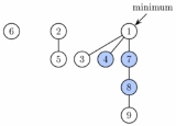
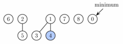
 Operation extract minimum (same as delete minimum) operates in three phases. First we take the root containing the minimum element and remove it. Its children will become roots of new trees. If the number of children was d, it takes time O(d) to process all new roots and the potential increases by d−1. Therefore the amortized running time of this phase is O(d) = O(log n).
 However to complete the extract minimum operation, we need to update the pointer to the root with minimum key. Unfortunately there may be up to n roots we need to check. In the second phase we therefore decrease the number of roots by successively linking together roots of the same degree. When two roots u and v have the same degree, we make one of them a child of the other so that the one with the smaller key remains the root. Its degree will increase by one. This is repeated until every root has a different degree. To find trees of the same degree efficiently we use an array of length O(log n) in which we keep a pointer to one root of each degree. When a second root is found of the same degree, the two are linked and the array is updated. The actual running time is O(log n + m) where m is the number of roots at the beginning of the second phase. At the end we will have at most O(log n) roots (because each has a different degree). Therefore the difference in the potential function from before this phase to after it is: O(log n) − m, and the amortized running time is then at most O(log n + m) + O(log n) − m = O(log n). Since we can scale up the units of potential stored at insertion in each node by the constant factor in the O(m) part of the actual cost for this phase.
In the third phase we check each of the remaining roots and find the minimum. This takes O(log n) time and the potential does not change. The overall amortized running time of extract minimum is therefore O(log n).
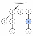
 Operation decrease key will take the node, decrease the key and if the heap property becomes violated (the new key is smaller than the key of the parent), the node is cut from its parent. If the parent is not a root, it is marked. If it has been marked already, it is cut as well and its parent is marked. We continue upwards until we reach either the root or an unmarked node. In the process we create some number, say k, of new trees. Each of these new trees except possibly the first one was marked originally but as a root it will become unmarked. One node can become marked. Therefore the potential decreases by at least k − 2. The actual time to perform the cutting was O(k), therefore the amortized running time is constant.
Finally, operation delete can be implemented simply by decreasing the key of the element to be deleted to minus infinity, thus turning it into the minimum of the whole heap. Then we call extract minimum to remove it. The amortized running time of this operation is O(log n).
. The degree bound follows from this and the fact (easily proved by induction) that for all integers
  , where
  . (We then have
  , and taking the log to base
  of both sides gives
  as required.)
Consider any node x somewhere in the heap (x need not be the root of one of the main trees). Define size(x) to be the size of the tree rooted at x (the number of descendants of x, including x itself). We prove by induction on the height of x (the length of a longest simple path from x to a descendant leaf), that size(x) ≥ Fd+2, where d is the degree of x.
Base case: If x has height 0, then d = 0, and size(x) = 1 = F2.
Inductive case: Suppose x has positive height and degree d>0. Let y1, y2, ..., yd be the children of x, indexed in order of the times they were most recently made children of x (y1 being the earliest and yd the latest), and let c1, c2, ..., cd be their respective degrees. We claim that ci ≥ i-2 for each i with 2≤i≤d: Just before yi was made a child of x, y1,...,yi−1 were already children of x, and so x had degree at least i−1 at that time. Since trees are combined only when the degrees of their roots are equal, it must have been that yi also had degree at least i-1 at the time it became a child of x. From that time to the present, yi can only have lost at most one child (as guaranteed by the marking process), and so its current degree ci is at least i−2. This proves the claim.
Since the heights of all the yi are strictly less than that of x, we can apply the inductive hypothesis to them to get size(yi) ≥ Fci+2 ≥ F(i−2)+2 = Fi. The nodes x and y1 each contribute at least 1 to size(x), and so we have

A routine induction proves that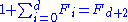 for any
  , which gives the desired lower bound on size(x).
.
(*)Amortized time
(**)With trivial modification to store an additional pointer to the minimum element
(***)Where n is the size of the larger heap
Computer science
Computer science or computing science is the study of the theoretical foundations of information and computation and of practical techniques for their implementation and application in computer systems...
, a Fibonacci heap is a heap data structure
Heap (data structure)
In computer science, a heap is a specialized tree-based data structure that satisfies the heap property: if B is a child node of A, then key ≥ key. This implies that an element with the greatest key is always in the root node, and so such a heap is sometimes called a max-heap...
consisting of a collection of tree
Tree (data structure)
In computer science, a tree is a widely-used data structure that emulates a hierarchical tree structure with a set of linked nodes.Mathematically, it is an ordered directed tree, more specifically an arborescence: an acyclic connected graph where each node has zero or more children nodes and at...
s. It has a better amortized
Amortized analysis
In computer science, amortized analysis is a method of analyzing algorithms that considers the entire sequence of operations of the program. It allows for the establishment of a worst-case bound for the performance of an algorithm irrespective of the inputs by looking at all of the operations...
running time than a binomial heap
Binomial heap
In computer science, a binomial heap is a heap similar to a binary heap but also supports quickly merging two heaps. This is achieved by using a special tree structure...
. Fibonacci heaps were developed by Michael L. Fredman
Michael Fredman
Michael Lawrence Fredman is a professor at the Computer Science Department at Rutgers University, United States. He got his Ph. D. degree from Stanford University in 1972 under the supervision of Donald Knuth. He was a member of the mathematics department at the Massachusetts Institute of...
and Robert E. Tarjan
Robert Tarjan
Robert Endre Tarjan is a renowned American computer scientist. He is the discoverer of several important graph algorithms, including Tarjan's off-line least common ancestors algorithm, and co-inventor of both splay trees and Fibonacci heaps. Tarjan is currently the James S...
in 1984 and first published in a scientific journal in 1987. The name of Fibonacci heap comes from Fibonacci number
Fibonacci number
In mathematics, the Fibonacci numbers are the numbers in the following integer sequence:0,\;1,\;1,\;2,\;3,\;5,\;8,\;13,\;21,\;34,\;55,\;89,\;144,\; \ldots\; ....
s which are used in the running time analysis.
Find-minimum is O(1) amortized time. Operations insert, decrease key, and merge (union) work in constant amortized time. Operations delete and delete minimum work in O
Big O notation
In mathematics, big O notation is used to describe the limiting behavior of a function when the argument tends towards a particular value or infinity, usually in terms of simpler functions. It is a member of a larger family of notations that is called Landau notation, Bachmann-Landau notation, or...
(log n) amortized time. This means that starting from an empty data structure, any sequence of a operations from the first group and b operations from the second group would take O(a + b log n) time. In a binomial heap such a sequence of operations would take O((a + b)log (n)) time. A Fibonacci heap is thus better than a binomial heap when b is asymptotically
Asymptotic analysis
In mathematical analysis, asymptotic analysis is a method of describing limiting behavior. The methodology has applications across science. Examples are...
smaller than a.
Using Fibonacci heaps for priority queue
Priority queue
A priority queue is an abstract data type in computer programming.It is exactly like a regular queue or stack data structure, but additionally, each element is associated with a "priority"....
s improves the asymptotic running time of important algorithms, such as Dijkstra's algorithm
Dijkstra's algorithm
Dijkstra's algorithm, conceived by Dutch computer scientist Edsger Dijkstra in 1956 and published in 1959, is a graph search algorithm that solves the single-source shortest path problem for a graph with nonnegative edge path costs, producing a shortest path tree...
for computing Shortest paths.
Structure
However at some point some order needs to be introduced to the heap to achieve the desired running time. In particular, degrees of nodes (here degree means the number of children) are kept quite low: every node has degree at most O(log n) and the size of a subtree rooted in a node of degree k is at least Fk + 2, where Fk is the kth Fibonacci number
Fibonacci number
In mathematics, the Fibonacci numbers are the numbers in the following integer sequence:0,\;1,\;1,\;2,\;3,\;5,\;8,\;13,\;21,\;34,\;55,\;89,\;144,\; \ldots\; ....
. This is achieved by the rule that we can cut at most one child of each non-root node. When a second child is cut, the node itself needs to be cut from its parent and becomes the root of a new tree (see Proof of degree bounds, below). The number of trees is decreased in the operation delete minimum, where trees are linked together.
As a result of a relaxed structure, some operations can take a long time while others are done very quickly. In the amortized running time
Amortized analysis
In computer science, amortized analysis is a method of analyzing algorithms that considers the entire sequence of operations of the program. It allows for the establishment of a worst-case bound for the performance of an algorithm irrespective of the inputs by looking at all of the operations...
analysis we pretend that very fast operations take a little bit longer than they actually do. This additional time is then later subtracted from the actual running time of slow operations. The amount of time saved for later use is measured at any given moment by a potential function. The potential of a Fibonacci heap is given by
- Potential = t + 2m
where t is the number of trees in the Fibonacci heap, and m is the number of marked nodes. A node is marked if at least one of its children was cut since this node was made a child of another node (all roots are unmarked).
Thus, the root of each tree in a heap has one unit of time stored. This unit of time can be used later to link this tree with another tree at amortized time 0. Also, each marked node has two units of time stored. One can be used to cut the node from its parent. If this happens, the node becomes a root and the second unit of time will remain stored in it as in any other root.
Implementation of operations
To allow fast deletion and concatenation, the roots of all trees are linked using a circular, doubly linked list. The children of each node are also linked using such a list. For each node, we maintain its number of children and whether the node is marked. Moreover we maintain a pointer to the root containing the minimum key.Operation find minimum is now trivial because we keep the pointer to the node containing it. It does not change the potential of the heap, therefore both actual and amortized cost is constant. As mentioned above, merge is implemented simply by concatenating the lists of tree roots of the two heaps. This can be done in constant time and the potential does not change, leading again to constant amortized time.
Operation insert works by creating a new heap with one element and doing merge. This takes constant time, and the potential increases by one, because the number of trees increases. The amortized cost is thus still constant.
In the third phase we check each of the remaining roots and find the minimum. This takes O(log n) time and the potential does not change. The overall amortized running time of extract minimum is therefore O(log n).
Finally, operation delete can be implemented simply by decreasing the key of the element to be deleted to minus infinity, thus turning it into the minimum of the whole heap. Then we call extract minimum to remove it. The amortized running time of this operation is O(log n).
Proof of degree bounds
The amortized performance of a Fibonacci heap depends on the degree (number of children) of any tree root being O(log n), where n is the size of the heap. Here we show that the size of the (sub)tree rooted at any node x of degree d in the heap must have size at least Fd+2, where Fk is the kth Fibonacci numberFibonacci number
In mathematics, the Fibonacci numbers are the numbers in the following integer sequence:0,\;1,\;1,\;2,\;3,\;5,\;8,\;13,\;21,\;34,\;55,\;89,\;144,\; \ldots\; ....
. The degree bound follows from this and the fact (easily proved by induction) that
for all integers , where . (We then have , and taking the log to base of both sides gives as required.)Consider any node x somewhere in the heap (x need not be the root of one of the main trees). Define size(x) to be the size of the tree rooted at x (the number of descendants of x, including x itself). We prove by induction on the height of x (the length of a longest simple path from x to a descendant leaf), that size(x) ≥ Fd+2, where d is the degree of x.
Base case: If x has height 0, then d = 0, and size(x) = 1 = F2.
Inductive case: Suppose x has positive height and degree d>0. Let y1, y2, ..., yd be the children of x, indexed in order of the times they were most recently made children of x (y1 being the earliest and yd the latest), and let c1, c2, ..., cd be their respective degrees. We claim that ci ≥ i-2 for each i with 2≤i≤d: Just before yi was made a child of x, y1,...,yi−1 were already children of x, and so x had degree at least i−1 at that time. Since trees are combined only when the degrees of their roots are equal, it must have been that yi also had degree at least i-1 at the time it became a child of x. From that time to the present, yi can only have lost at most one child (as guaranteed by the marking process), and so its current degree ci is at least i−2. This proves the claim.
Since the heights of all the yi are strictly less than that of x, we can apply the inductive hypothesis to them to get size(yi) ≥ Fci+2 ≥ F(i−2)+2 = Fi. The nodes x and y1 each contribute at least 1 to size(x), and so we have
A routine induction proves that
for any , which gives the desired lower bound on size(x).Worst case
Although the total running time of a sequence of operations starting with an empty structure is bounded by the bounds given above, some (very few) operations in the sequence can take very long to complete (in particular delete and delete minimum have linear running time in the worst case). For this reason Fibonacci heaps and other amortized data structures may not be appropriate for real-time systemsReal-time computing
In computer science, real-time computing , or reactive computing, is the study of hardware and software systems that are subject to a "real-time constraint"— e.g. operational deadlines from event to system response. Real-time programs must guarantee response within strict time constraints...
.
Summary of running times
| Common Operations | Effect | Unsorted Linked List Linked list In computer science, a linked list is a data structure consisting of a group of nodes which together represent a sequence. Under the simplest form, each node is composed of a datum and a reference to the next node in the sequence; more complex variants add additional links... |
Self-balancing binary search tree Self-balancing binary search tree In computer science, a self-balancing binary search tree is any node based binary search tree that automatically keeps its height small in the face of arbitrary item insertions and deletions.... |
Binary heap Binary heap A binary heap is a heap data structure created using a binary tree. It can be seen as a binary tree with two additional constraints:*The shape property: the tree is a complete binary tree; that is, all levels of the tree, except possibly the last one are fully filled, and, if the last level of... |
Binomial heap Binomial heap In computer science, a binomial heap is a heap similar to a binary heap but also supports quickly merging two heaps. This is achieved by using a special tree structure... |
Fibonacci heap | Brodal queue Brodal queue In computer science, the Brodal queue is a heap/priority queue structure with very low worst case time bounds: O for insertion, find-minimum, meld and decrease-key and O for delete-minimum and general deletion; they are the first heap variant with these bounds... |
Pairing heap Pairing heap A pairing heaps is a type of heap data structure with relatively simple implementation and excellent practical amortized performance. However, it has proven very difficult to determine the precise asymptotic running time of pairing heaps.... |
|---|---|---|---|---|---|---|---|---|
| insert(data,key) | Adds data to the queue, tagged with key | O(1) | O(log n) | O(log n) | O(log n) | O(1) | O(1) | O(1) |
| findMin -> key,data | Returns key,data corresponding to min-value key | O(n) | O(log n) or O(1) (**) | O(1) | O(log n) | O(1) | O(1) | O(1) |
| deleteMin | Deletes data corresponding to min-value key | O(n) | O(log n) | O(log n) | O(log n) | O(log n)* | O(log n) | O(log n)} |
| delete(node) | Deletes data corresponding to given key, given a pointer to the node being deleted | O(1) | O(log n) | O(log n) | O(log n) | O(log n)* | O(log n) | O(log n)} |
| decreaseKey(node) | Decreases the key of a node, given a pointer to the node being modified | O(1) | O(log n) | O(log n) | O(log n) | O(1)* | O(1) | Unknown but bounded: 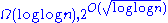 } } |
| merge(heap1,heap2) -> heap3 | Merges two heaps into a third | O(1) | O(m log(n+m)) | O(m + n) | O(log n)*** | O(1) | O(1) | O(1) |
(*)Amortized time
(**)With trivial modification to store an additional pointer to the minimum element
(***)Where n is the size of the larger heap
External links
- Java applet simulation of a Fibonacci heap
- C implementation of Fibonacci heap
- MATLAB implementation of Fibonacci heap
- De-recursived and memory efficient C implementation of Fibonacci heap (free/libre software, CeCILL-B license)
- C++ template Fibonacci heap, with demonstration
- Ruby implementation of the Fibonacci heap (with tests)
- Pseudocode of the Fibonacci heap algorithm