
Approximation theory
Encyclopedia
In mathematics
, approximation theory is concerned with how function
s can best be approximated
with simpler functions
, and with quantitative
ly characterizing
the errors
introduced thereby. Note that what is meant by best and simpler will depend on the application.
A closely related topic is the approximation of functions by generalized Fourier series
, that is, approximations based upon summation of a series of terms based upon orthogonal polynomials
.
One problem of particular interest is that of approximating a function in a computer
mathematical library, using operations that can be performed on the computer or calculator (e.g. addition and multiplication), such that the result is as close to the actual function as possible. This is typically done with polynomial
or rational
(ratio of polynomials) approximations.
The objective is to make the approximation as close as possible to the actual function, typically with an accuracy close to that of the underlying computer's floating point
arithmetic. This is accomplished by using a polynomial of high degree
, and/or narrowing the domain over which the polynomial has to approximate the function.
Narrowing the domain can often be done through the use of various addition or scaling formulas for the function being approximated. Modern mathematical libraries often reduce the domain into many tiny segments and use a low-degree polynomial for each segment.
 , where P(x) is the approximating polynomial and f(x) is the actual function. For well-behaved functions, there exists an Nth-degree polynomial that will lead to an error curve that oscillates back and forth between
  and
and  a total of N+2 times, giving a worst-case error of
  . It is seen that an Nth-degree polynomial can interpolate N+1 points in a curve. Such a polynomial is always optimal. It is possible to make contrived functions f(x) for which no such polynomial exists, but these occur rarely in practice.
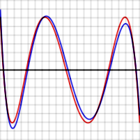
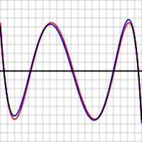
For example the graphs shown to the right show the error in approximating log(x) and exp(x) for N = 4. The red curves, for the optimal polynomial, are level, that is, they oscillate between and
and  exactly. Note that, in each case, the number of extrema is N+2, that is, 6. Two of the extrema are at the end points of the interval, at the left and right edges of the graphs.
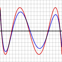 To prove this is true in general, suppose P is a polynomial of degree N having the property described, that is, it gives rise to an error function that has N + 2 extrema, of alternating signs and equal magnitudes. The red graph to the right shows what this error function might look like for N = 4. Suppose Q(x) (whose error function is shown in blue to the right) is another N-degree polynomial that is a better approximation to f than P. In particular, Q is closer to f than P for each value xi where an extreme of P−f occurs, so
When a maximum of P−f occurs at xi, then
And when a minimum of P−f occurs at xi, then
So, as can be seen in the graph, [P(x) − f(x)] − [Q(x) − f(x)] must alternate in sign for the N + 2 values of xi. But [P(x) − f(x)] − [Q(x) − f(x)] reduces to P(x) − Q(x) which is a polynomial of degree N. This function changes sign at least N+1 times so, by the Intermediate value theorem
, it has N+1 zeroes, which is impossible for a polynomial of degree N.
and then cutting off the expansion at the desired degree.
This is similar to the Fourier analysis
of the function, using the Chebyshev polynomials instead of the usual trigonometric functions.
If one calculates the coefficients in the Chebyshev expansion for a function:

and then cuts off the series after the term, one gets an Nth-degree polynomial approximating f(x).
The reason this polynomial is nearly optimal is that, for functions with rapidly converging power series, if the series is cut off after some term, the total error arising from the cutoff is close to the first term after the cutoff. That is, the first term after the cutoff dominates all later terms. The same is true if the expansion is in terms of Chebyshev polynomials. If a Chebyshev expansion is cut off after , the error will take a form close to a multiple of
  . The Chebyshev polynomials have the property that they are level – they oscillate between +1 and −1 in the interval [−1, 1].
  has N+2 level extrema. This means that the error between f(x) and its Chebyshev expansion out to
  is close to a level function with N+2 extrema, so it is close to the optimal Nth-degree polynomial.
In the graphs above, note that the blue error function is sometimes better than (inside of) the red function, but sometimes worse, meaning that it is not quite the optimal polynomial. Note also that the discrepancy is less serious for the exp function, which has an extremely rapid converging power series, than for the log function.
Chebyshev approximation is the basis for Clenshaw–Curtis quadrature, a numerical integration
technique.
(sometimes spelled Remes) is used to produce an optimal polynomial P(x) approximating a given function f(x) over a given interval. It is an iterative algorithm that converges to a polynomial that has an error function with N+2 level extrema. By the theorem above, that polynomial is optimal.
Remez' algorithm uses the fact that one can construct an Nth-degree polynomial that leads to level and alternating error values, given N+2 test points.
Given N+2 test points ,
,  ...
...  (where
  and
and  are presumably the end points of the interval of approximation), these equations need to be solved:


The right-hand sides alternate in sign.
That is,


Since ...
...  were given, all of their powers are known, and
  ...
...  are also known. That means that the above equations are just N+2 linear equations in the N+2 variables
  ,
,  ...
...  , and
, and  . Given the test points
  ...
...  , one can solve this system to get the polynomial P and the number
  .
.
The graph below shows an example of this, producing a 4th degree polynomial approximating over [−1, 1]. The test points were set at
−1, −0.7, −0.1, +0.4, +0.9, and 1. Those values are shown in green. The resultant value of is 4.43 x 10⁻⁴
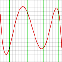 Note that the error graph does indeed take on the values
  at the 6 test points, including the end points, but that those points are not extrema. If the 4 interior test points had been extrema (that is, the function P(x)f(x) had maxima or minima there), the polynomial would be optimal.
The second step of Remez' algorithm consists of moving the test points to the approximate locations where the error function had its actual local maxima or minima. For example, one can tell from looking at the graph that the point at −0.1 should have been at about −0.28.
The way to do this in the algorithm is to use a single round of
Newton's method
. Since one knows the first and second derivatives of P(x)−f(x), one can calculate approximately how far a test point has to be moved so that the derivative will be zero.
After moving the test points, the linear equation part is repeated, getting a new polynomial, and Newton's method is used again to move the test points again. This sequence is continued until the result converges to the desired accuracy. The algorithm converges very rapidly.
Convergence is quadratic for well-behaved functions—if the test points are within of the correct result, they will be approximately within
  of the correct result after the next round.
Remez' algorithm is typically started by choosing the extrema of the Chebyshev polynomial as the initial points, since the final error function will be similar to that polynomial.
Mathematics
Mathematics is the study of quantity, space, structure, and change. Mathematicians seek out patterns and formulate new conjectures. Mathematicians resolve the truth or falsity of conjectures by mathematical proofs, which are arguments sufficient to convince other mathematicians of their validity...
, approximation theory is concerned with how function
Function (mathematics)
In mathematics, a function associates one quantity, the argument of the function, also known as the input, with another quantity, the value of the function, also known as the output. A function assigns exactly one output to each input. The argument and the value may be real numbers, but they can...
s can best be approximated
Approximation
An approximation is a representation of something that is not exact, but still close enough to be useful. Although approximation is most often applied to numbers, it is also frequently applied to such things as mathematical functions, shapes, and physical laws.Approximations may be used because...
with simpler functions
Function (mathematics)
In mathematics, a function associates one quantity, the argument of the function, also known as the input, with another quantity, the value of the function, also known as the output. A function assigns exactly one output to each input. The argument and the value may be real numbers, but they can...
, and with quantitative
Quantitative property
A quantitative property is one that exists in a range of magnitudes, and can therefore be measured with a number. Measurements of any particular quantitative property are expressed as a specific quantity, referred to as a unit, multiplied by a number. Examples of physical quantities are distance,...
ly characterizing
Characterization (mathematics)
In mathematics, the statement that "Property P characterizes object X" means, not simply that X has property P, but that X is the only thing that has property P. It is also common to find statements such as "Property Q characterises Y up to isomorphism". The first type of statement says in...
the errors
Approximation error
The approximation error in some data is the discrepancy between an exact value and some approximation to it. An approximation error can occur because#the measurement of the data is not precise due to the instruments...
introduced thereby. Note that what is meant by best and simpler will depend on the application.
A closely related topic is the approximation of functions by generalized Fourier series
Generalized Fourier series
In mathematical analysis, many generalizations of Fourier series have proved to be useful.They are all special cases of decompositions over an orthonormal basis of an inner product space....
, that is, approximations based upon summation of a series of terms based upon orthogonal polynomials
Orthogonal polynomials
In mathematics, the classical orthogonal polynomials are the most widely used orthogonal polynomials, and consist of the Hermite polynomials, the Laguerre polynomials, the Jacobi polynomials together with their special cases the ultraspherical polynomials, the Chebyshev polynomials, and the...
.
One problem of particular interest is that of approximating a function in a computer
Computer
A computer is a programmable machine designed to sequentially and automatically carry out a sequence of arithmetic or logical operations. The particular sequence of operations can be changed readily, allowing the computer to solve more than one kind of problem...
mathematical library, using operations that can be performed on the computer or calculator (e.g. addition and multiplication), such that the result is as close to the actual function as possible. This is typically done with polynomial
Polynomial
In mathematics, a polynomial is an expression of finite length constructed from variables and constants, using only the operations of addition, subtraction, multiplication, and non-negative integer exponents...
or rational
Rational function
In mathematics, a rational function is any function which can be written as the ratio of two polynomial functions. Neither the coefficients of the polynomials nor the values taken by the function are necessarily rational.-Definitions:...
(ratio of polynomials) approximations.
The objective is to make the approximation as close as possible to the actual function, typically with an accuracy close to that of the underlying computer's floating point
Floating point
In computing, floating point describes a method of representing real numbers in a way that can support a wide range of values. Numbers are, in general, represented approximately to a fixed number of significant digits and scaled using an exponent. The base for the scaling is normally 2, 10 or 16...
arithmetic. This is accomplished by using a polynomial of high degree
Degree of a polynomial
The degree of a polynomial represents the highest degree of a polynominal's terms , should the polynomial be expressed in canonical form . The degree of an individual term is the sum of the exponents acting on the term's variables...
, and/or narrowing the domain over which the polynomial has to approximate the function.
Narrowing the domain can often be done through the use of various addition or scaling formulas for the function being approximated. Modern mathematical libraries often reduce the domain into many tiny segments and use a low-degree polynomial for each segment.
 |
 |
Optimal polynomials
Once the domain and degree of the polynomial are chosen, the polynomial itself is chosen in such a way as to minimize the worst-case error. That is, the goal is to minimize the maximum value of , where P(x) is the approximating polynomial and f(x) is the actual function. For well-behaved functions, there exists an Nth-degree polynomial that will lead to an error curve that oscillates back and forth between
  and
and  a total of N+2 times, giving a worst-case error of
  . It is seen that an Nth-degree polynomial can interpolate N+1 points in a curve. Such a polynomial is always optimal. It is possible to make contrived functions f(x) for which no such polynomial exists, but these occur rarely in practice.
For example the graphs shown to the right show the error in approximating log(x) and exp(x) for N = 4. The red curves, for the optimal polynomial, are level, that is, they oscillate between
 and
and  exactly. Note that, in each case, the number of extrema is N+2, that is, 6. Two of the extrema are at the end points of the interval, at the left and right edges of the graphs.

When a maximum of P−f occurs at xi, then

And when a minimum of P−f occurs at xi, then

So, as can be seen in the graph, [P(x) − f(x)] − [Q(x) − f(x)] must alternate in sign for the N + 2 values of xi. But [P(x) − f(x)] − [Q(x) − f(x)] reduces to P(x) − Q(x) which is a polynomial of degree N. This function changes sign at least N+1 times so, by the Intermediate value theorem
Intermediate value theorem
In mathematical analysis, the intermediate value theorem states that for each value between the least upper bound and greatest lower bound of the image of a continuous function there is at least one point in its domain that the function maps to that value....
, it has N+1 zeroes, which is impossible for a polynomial of degree N.
Chebyshev approximation
One can obtain polynomials very close to the optimal one by expanding the given function in terms of Chebyshev polynomialsChebyshev polynomials
In mathematics the Chebyshev polynomials, named after Pafnuty Chebyshev, are a sequence of orthogonal polynomials which are related to de Moivre's formula and which can be defined recursively. One usually distinguishes between Chebyshev polynomials of the first kind which are denoted Tn and...
and then cutting off the expansion at the desired degree.
This is similar to the Fourier analysis
Harmonic analysis
Harmonic analysis is the branch of mathematics that studies the representation of functions or signals as the superposition of basic waves. It investigates and generalizes the notions of Fourier series and Fourier transforms...
of the function, using the Chebyshev polynomials instead of the usual trigonometric functions.
If one calculates the coefficients in the Chebyshev expansion for a function:

and then cuts off the series after the
 term, one gets an Nth-degree polynomial approximating f(x).
The reason this polynomial is nearly optimal is that, for functions with rapidly converging power series, if the series is cut off after some term, the total error arising from the cutoff is close to the first term after the cutoff. That is, the first term after the cutoff dominates all later terms. The same is true if the expansion is in terms of Chebyshev polynomials. If a Chebyshev expansion is cut off after
 , the error will take a form close to a multiple of
  . The Chebyshev polynomials have the property that they are level – they oscillate between +1 and −1 in the interval [−1, 1].
  has N+2 level extrema. This means that the error between f(x) and its Chebyshev expansion out to
  is close to a level function with N+2 extrema, so it is close to the optimal Nth-degree polynomial.
In the graphs above, note that the blue error function is sometimes better than (inside of) the red function, but sometimes worse, meaning that it is not quite the optimal polynomial. Note also that the discrepancy is less serious for the exp function, which has an extremely rapid converging power series, than for the log function.
Chebyshev approximation is the basis for Clenshaw–Curtis quadrature, a numerical integration
Numerical integration
In numerical analysis, numerical integration constitutes a broad family of algorithms for calculating the numerical value of a definite integral, and by extension, the term is also sometimes used to describe the numerical solution of differential equations. This article focuses on calculation of...
technique.
Remez' algorithm
The Remez algorithmRemez algorithm
The Remez algorithm , published by Evgeny Yakovlevich Remez in 1934 is an iterative algorithm used to find simple approximations to functions, specifically, approximations by functions in a Chebyshev space that are the best in the uniform norm L∞ sense.A typical...
(sometimes spelled Remes) is used to produce an optimal polynomial P(x) approximating a given function f(x) over a given interval. It is an iterative algorithm that converges to a polynomial that has an error function with N+2 level extrema. By the theorem above, that polynomial is optimal.
Remez' algorithm uses the fact that one can construct an Nth-degree polynomial that leads to level and alternating error values, given N+2 test points.
Given N+2 test points
 ,
,  ...
...  (where
  and
and  are presumably the end points of the interval of approximation), these equations need to be solved:


The right-hand sides alternate in sign.
That is,


Since
 ...
...  were given, all of their powers are known, and
  ...
...  are also known. That means that the above equations are just N+2 linear equations in the N+2 variables
  ,
,  ...
...  , and
, and  . Given the test points
  ...
...  , one can solve this system to get the polynomial P and the number
  .
.The graph below shows an example of this, producing a 4th degree polynomial approximating
 over [−1, 1]. The test points were set at
−1, −0.7, −0.1, +0.4, +0.9, and 1. Those values are shown in green. The resultant value of
 is 4.43 x 10⁻⁴
 at the 6 test points, including the end points, but that those points are not extrema. If the 4 interior test points had been extrema (that is, the function P(x)f(x) had maxima or minima there), the polynomial would be optimal.
The second step of Remez' algorithm consists of moving the test points to the approximate locations where the error function had its actual local maxima or minima. For example, one can tell from looking at the graph that the point at −0.1 should have been at about −0.28.
The way to do this in the algorithm is to use a single round of
Newton's method
Newton's method
In numerical analysis, Newton's method , named after Isaac Newton and Joseph Raphson, is a method for finding successively better approximations to the roots of a real-valued function. The algorithm is first in the class of Householder's methods, succeeded by Halley's method...
. Since one knows the first and second derivatives of P(x)−f(x), one can calculate approximately how far a test point has to be moved so that the derivative will be zero.
- Calculating the derivatives of a polynomial is straightforward. One must also be able to calculate the first and second derivatives of f(x). Remez' algorithm requires an ability to calculate
 ,
,  , and
, and  to extremely high precision. The entire algorithm must be carried out to higher precision than the desired precision of the result.
After moving the test points, the linear equation part is repeated, getting a new polynomial, and Newton's method is used again to move the test points again. This sequence is continued until the result converges to the desired accuracy. The algorithm converges very rapidly.
Convergence is quadratic for well-behaved functions—if the test points are within
 of the correct result, they will be approximately within
  of the correct result after the next round.
Remez' algorithm is typically started by choosing the extrema of the Chebyshev polynomial
 as the initial points, since the final error function will be similar to that polynomial.
Main journals
- Journal of Approximation TheoryJournal of Approximation TheoryThe Journal of Approximation Theory is "devoted to advances in pure and applied approximation theory and related areas."...
- Constructive ApproximationConstructive ApproximationConstructive Approximation is "an international mathematics journal dedicated to Approximations and Expansions and related research in computation, function theory, functional analysis, interpolation spaces and interpolation of operators, numerical analysis, space of functions, special functions,...
- East Journal on ApproximationsEast Journal on ApproximationsThe East Journal on Approximations is a journal about approximation theory published in Sofia, Bulgaria....
See also
- Chebyshev polynomialsChebyshev polynomialsIn mathematics the Chebyshev polynomials, named after Pafnuty Chebyshev, are a sequence of orthogonal polynomials which are related to de Moivre's formula and which can be defined recursively. One usually distinguishes between Chebyshev polynomials of the first kind which are denoted Tn and...
- Generalized Fourier seriesGeneralized Fourier seriesIn mathematical analysis, many generalizations of Fourier series have proved to be useful.They are all special cases of decompositions over an orthonormal basis of an inner product space....
- Orthogonal polynomialsOrthogonal polynomialsIn mathematics, the classical orthogonal polynomials are the most widely used orthogonal polynomials, and consist of the Hermite polynomials, the Laguerre polynomials, the Jacobi polynomials together with their special cases the ultraspherical polynomials, the Chebyshev polynomials, and the...
- Orthonormal basisOrthonormal basisIn mathematics, particularly linear algebra, an orthonormal basis for inner product space V with finite dimension is a basis for V whose vectors are orthonormal. For example, the standard basis for a Euclidean space Rn is an orthonormal basis, where the relevant inner product is the dot product of...
- Fourier seriesFourier seriesIn mathematics, a Fourier series decomposes periodic functions or periodic signals into the sum of a set of simple oscillating functions, namely sines and cosines...
- Schauder basisSchauder basisIn mathematics, a Schauder basis or countable basis is similar to the usual basis of a vector space; the difference is that Hamel bases use linear combinations that are finite sums, while for Schauder bases they may be infinite sums...
- Padé approximantPadé approximantPadé approximant is the "best" approximation of a function by a rational function of given order - under this technique, the approximant's power series agrees with the power series of the function it is approximating....

