
SIMCOS
Encyclopedia
Development environment
In hosted software development, a development environment refers to a server tier designated to a specific stage in a release process....
for computer simulation
Computer simulation
A computer simulation, a computer model, or a computational model is a computer program, or network of computers, that attempts to simulate an abstract model of a particular system...
. In 1989 it was developed by Slovenian
Slovenians
The Slovenes, Slovene people, Slovenians, or Slovenian people are a South Slavic people primarily associated with Slovenia and the Slovene language.-Population:Most Slovenes today live within the borders of the independent Slovenia...
experts led by Borut Zupančič.
Properties
The purpose of the language is simulationSimulation
Simulation is the imitation of some real thing available, state of affairs, or process. The act of simulating something generally entails representing certain key characteristics or behaviours of a selected physical or abstract system....
of dynamic mathematical model
Mathematical model
A mathematical model is a description of a system using mathematical concepts and language. The process of developing a mathematical model is termed mathematical modeling. Mathematical models are used not only in the natural sciences and engineering disciplines A mathematical model is a...
s of systems, given as set of ordinary differential equation
Ordinary differential equation
In mathematics, an ordinary differential equation is a relation that contains functions of only one independent variable, and one or more of their derivatives with respect to that variable....
s. It is an equation oriented and compiler type of language. Despite its name it can be used for discrete simulation as well. The language suits well to the CSSL'67 standard of simulation languages so portability among other languages conforming to the same standard (e.g. Tutsim, ACSL
Advanced Continuous Simulation Language
The Advanced Continuous Simulation Language, or ACSL , is a computer language designed for modelling and evaluating the performance of continuous systems described by time-dependent, nonlinear differential equations...
etc.) is quite simple. It is a DOS
DOS
DOS, short for "Disk Operating System", is an acronym for several closely related operating systems that dominated the IBM PC compatible market between 1981 and 1995, or until about 2000 if one includes the partially DOS-based Microsoft Windows versions 95, 98, and Millennium Edition.Related...
based software occasionally it is slightly modified so it can be run under actual versions of Microsoft Windows
Microsoft Windows
Microsoft Windows is a series of operating systems produced by Microsoft.Microsoft introduced an operating environment named Windows on November 20, 1985 as an add-on to MS-DOS in response to the growing interest in graphical user interfaces . Microsoft Windows came to dominate the world's personal...
. Apart from the simulation itself it can also perform parametrisation (a series of simulations with different values of parameter
Parameter
Parameter from Ancient Greek παρά also “para” meaning “beside, subsidiary” and μέτρον also “metron” meaning “measure”, can be interpreted in mathematics, logic, linguistics, environmental science and other disciplines....
s), linearisation of models and optimisation
Optimization (mathematics)
In mathematics, computational science, or management science, mathematical optimization refers to the selection of a best element from some set of available alternatives....
(finding such values of parameters that a criterion function is minimised).
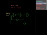
Simulation process
When a simulation scheme must be prepared it must be described in the SIMCOS language. It can be "drawn" (similarly as with an analogue computer) using an enclosed block library graphics tool (it contains basic elements such as integratorIntegrator
An integrator is a device to perform the mathematical operation known as integration, a fundamental operation in calculus.The integration function is often part of engineering, physics, mechanical, chemical and scientific calculations....
s, amplifier
Amplifier
Generally, an amplifier or simply amp, is a device for increasing the power of a signal.In popular use, the term usually describes an electronic amplifier, in which the input "signal" is usually a voltage or a current. In audio applications, amplifiers drive the loudspeakers used in PA systems to...
s, summators, some basic input signals etc.) but more often it is entered as a program using one of text editors, e.g. Edit enclosed with MS DOS. Whichever form of entry of the model is used, the first phase of simulation reprocesses it into space of states form and rewrites the program into Fortran
Fortran
Fortran is a general-purpose, procedural, imperative programming language that is especially suited to numeric computation and scientific computing...
and prepares files with input parameters. This Fortran program is compiled into an executable file (.EXE) and executed. The executable program reads parameter values from input files, performs the simulation and writes requested calculated values into another file. When it terminates, SIMCOS takes control again and can display results as a graphic plot.
The "heart" of the executable is function INTEG which can solve differential equation
Differential equation
A differential equation is a mathematical equation for an unknown function of one or several variables that relates the values of the function itself and its derivatives of various orders...
s using one of several numerical methods. First it reads necessary values (e.g. values of parameters, initial conditions) from files then it calls the function DERIV where the model is actually described as series of functions of its derivative
Derivative
In calculus, a branch of mathematics, the derivative is a measure of how a function changes as its input changes. Loosely speaking, a derivative can be thought of as how much one quantity is changing in response to changes in some other quantity; for example, the derivative of the position of a...
s. The returned values are used at the selected numerical method. Requested calculated results are written into the file and the whole procedure is repeated until the termination condition is satisfied.
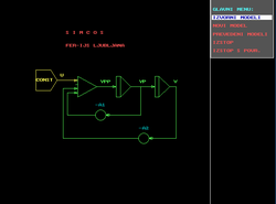
Example
Continuous simulation of dead timeDead time
For detection systems that record discrete events, such as particle and nuclear detectors, the dead time is the time after each event during which the system is not able to record another event....
(its Laplace transform is
 ) is not a trivial task and usually we use one of Padé approximations. We will simulate Padé approximation of 2nd order
and 4th order:

Input signal is a unit step, communication interval equals 0.01s, length simulation run is 5s, results will be compared with output of built-in discrete function delay (it requires additional array (del in our case) of appropriate size).
y1 is a result of simulation of Padé approximation of 2nd order, y2 is a result of simulation of Padé approximation of 4th order and y3 is result of the discrete function delay.
When transfer function
Transfer function
A transfer function is a mathematical representation, in terms of spatial or temporal frequency, of the relation between the input and output of a linear time-invariant system. With optical imaging devices, for example, it is the Fourier transform of the point spread function i.e...
s of both Padé approximation are developed using one of simulation schemes, the model can be described with the following program:
program pade

constant tm=1.0

constant tfin=5

array del(101)

variable t=0.0

u=step(t,0.)


u11d=12/(tm*tm)*u-12/(tm*tm)*y1

u11=integ(u11d,0.)

u21d=u11-u*6/tm-y1*6/tm

u21=integ(u21d,0.)

y1=u21+u

u12d=u*1680/(tm*tm*tm*tm)-y2*1680/(tm*tm*tm*tm)

u12=integ(u12d,0.)

u22d=u12-u*840/(tm*tm*tm)-y2*840/(tm*tm*tm)

u22=integ(u22d,0.)

u32d=u22+u*180/(tm*tm)-y2*180/(tm*tm)

u32=integ(u32d,0.)

u42d=u32-u*20/tm-y2*20*tm

u42=integ(u42d,0.)

y2=u42+u

y3=delay(u,tm,#del,ci)


cinterval ci=0.01

hdr Pade approximation of dead time

prepar y1,y2,y3

output 10,y1,y2,y3

termt(t.ge.tfin)


end

External links
- Borut Zupančič's homepage
- LMSC download page (the link to SIMCOS is at the bottom)