

Adiabatic theorem
Encyclopedia
The adiabatic theorem is an important concept in quantum mechanics
. Its original form, due to Max Born
and Vladimir Fock
(1928), can be stated as follows:
It may not be immediately clear from this formulation, but the adiabatic theorem is an extremely intuitive concept. Simply stated, a quantum mechanical system subjected to gradually changing external conditions can adapt its functional form, while in the case of rapidly varying conditions there is no time for the functional form of the state to adapt so the probability density remains unchanged.
The consequences of this apparently simple result are many, varied and extremely subtle. In order to make this clear we will begin with a fairly qualitative description, followed by a series of example systems, before undertaking a more rigorous analysis. Finally we will look at techniques used for adiabaticity calculations.
 a quantum-mechanical system has an energy given by the Hamiltonian
  ; the system is in an eigenstate of
  labelled
  . Changing conditions modify the Hamiltonian in a continuous manner, resulting in a final Hamiltonian
  at some later time
  . The system will evolve according to the Schrödinger equation, to reach a final state
  . The adiabatic theorem states that the modification to the system depends critically on the time
  during which the modification takes place.
For a truly adiabatic process we require ; in this case the final state
  will be an eigenstate of the final Hamiltonian
  , with a modified configuration:
 .
.
The degree to which a given change approximates an adiabatic process depends on both the energy separation between and adjacent states, and the ratio of the interval
  to the characteristic time-scale of the evolution of
  for a time-independent Hamiltonian,
  , where
  is the energy of
  .
.
Conversely, in the limit we have infinitely rapid, or diabatic passage; the configuration of the state remains unchanged:
 .
.
The so-called "gap condition" included in Born and Fock's original definition given above refers to a requirement that the spectrum of is discrete
and nondegenerate
, such that there is no ambiguity in the ordering of the states (one can easily establish which eigenstate of corresponds to
  ). In 1999 J. E. Avron and A. Elgart reformulated the adiabatic theorem, eliminating the gap condition.
Note that the term "adiabatic" is traditionally used in thermodynamics
to describe processes without the exchange of heat between system and environment (see adiabatic process
). The quantum mechanical definition is closer to the thermodynamical concept of a quasistatic process
, and has no direct relation with heat exchange.
oscillating in a vertical plane. If the support is moved, the mode of oscillation of the pendulum will change. If the support is moved sufficiently slowly, the motion of the pendulum relative to the support will remain unchanged. A gradual change in external conditions allows the system to adapt, such that it retains its initial character. This is referred to as an adiabatic process.
 The classical
nature of a pendulum precludes a full description of the effects of the adiabatic theorem. As a further example consider a quantum harmonic oscillator as the spring constant is increased. Classically this is equivalent to increasing the stiffness of a spring; quantum-mechanically the effect is a narrowing of the potential-energy curve in the system Hamiltonian
.
If is increased adiabatically
  then the system at time
  will be in an instantaneous eigenstate
  of the current Hamiltonian
  , corresponding to the initial eigenstate of
  . For the special case of a system like the quantum harmonic oscillator described by a single quantum number
, this means the quantum number will remain unchanged. Figure 1 shows how a harmonic oscillator, initially in its ground state, , remains in the ground state as the potential-energy curve is compressed; the functional form of the state adapting to the slowly varying conditions.
For a rapidly increased spring constant, the system undergoes a diabatic process in which the system has no time to adapt its functional form to the changing conditions. While the final state must look identical to the initial state
  for a process occurring over a vanishing time period, there is no eigenstate of the new Hamiltonian,
  , that resembles the initial state. The final state is composed of a linear superposition of many different eigenstates of
  which sum to reproduce the form of the initial state.
 For a more widely applicable example, consider a 2-level
atom subjected to an external magnetic field
. The states, labelled and
and  using bra-ket notation
, can be thought of as atomic angular-momentum states
, each with a particular geometry. For reasons that will become clear these states will henceforth be referred to as the diabatic states. The system wavefunction can be represented as a linear combination of the diabatic states:

With the field absent, the energetic separation of the diabatic states is equal to ; the energy of state
  increases with increasing magnetic field (a low-field-seeking state), while the energy of state
  decreases with increasing magnetic field (a high-field-seeking state). Assuming the magnetic-field dependence is linear, the Hamiltonian matrix for the system with the field applied can be written

where is the magnetic moment
of the atom, assumed to be the same for the two diabatic states, and is some time-independent coupling
between the two states. The diagonal elements are the energies of the diabatic states ( and
and  ), however, as
  is not a diagonal matrix
, it is clear that these states are not eigenstates of the new Hamiltonian that includes the magnetic field contribution.
The eigenvectors of the matrix are the eigenstates of the system, which we will label
  and
and  , with corresponding eigenvalues

It is important to realise that the eigenvalues and
and  are the only allowed outputs for any individual measurement of the system energy, whereas the diabatic energies
  and
and  correspond to the expectation values for the energy of the system in the diabatic states
  and
and  .
.
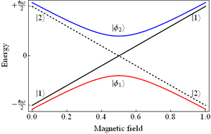
Figure 2 shows the dependence of the diabatic and adiabatic energies on the value of the magnetic field; note that for non-zero coupling the eigenvalues of the Hamiltonian cannot be degenerate
, and thus we have an avoided crossing. If an atom is initially in state in zero magnetic field (on the red curve, at the extreme left), an adiabatic increase in magnetic field
  will ensure the system remains in an eigenstate of the Hamiltonian
  throughout the process(follows the red curve). A diabatic increase in magnetic field
  will ensure the system follows the diabatic path (the solid black line), such that the system undergoes a transition to state
  . For finite magnetic field slew rates
  there will be a finite probability of finding the system in either of the two eigenstates. See below for approaches to calculating these probabilities.
These results are extremely important in atomic
and molecular physics
for control of the energy-state distribution in a population of atoms or molecules.
and Vladimir Fock
, in Zeitschrift für Physik 51, 165 (1928). The concept of this theorem deals with the time-dependent Hamiltonian
(which might be called a subject of Quantum dynamics
) where the Hamiltonian changes with time.
In adiabatic process the Hamiltonian is time-dependent i.e, the Hamiltonian changes with time (not to be confused with Perturbation theory
, as here the change in Hamiltonian is not small; it's huge, although it happens gradually). As because Hamiltonian changes with time, the eigenvalues and the eigenfunctions are time dependent.
But at any particular instant of time the states still gives Complete orthogonal system. i.e,
Notice that: The dependence on position is tactically suppressed, as the time dependence part will be in more concern. will considered to be the state of the system at time t no-matter how it depends on its position.
The general solution of time dependent Schrödinger equation now can be expressed as where
where  .
.
The phase is called the dynamic phase factor. By substitution into the Schrödinger equation, another equation for the variation of the coefficients can be obtained
The term gives
gives  and so the third term of left hand side cancels out with the right hand side leaving
now taking the inner product with an arbitrary eigenfunction , the on the left
  gives
gives  which is 1 only for m = n otherwise vanishes. The remaining part gives
calculating the expression for from differentiating the modified time independent Schrödinger equation above it can have the form
This is also exact.For the adiabatic approximation which says the time derivative of Hamiltonian i.e, is extremely small as time is largely taken, the last term will dropout and one has
that gives, after solving,
having defined the geometric phase
as . Putting it in the expression for nth eigenstate one has
So, for an adiabatic process, a particle starting from nth eigenstate also remains in that nth eigenstate like it does for the time-independent processes, only picking up a couple of phase factors. The new phase factor can be canceled out by an appropriate choice of gauge for the eigenfunctions. However, if the adiabatic evolution is cyclic, then
  becomes a gauge-invariant physical quantity, known as the Berry phase.
, the state vector of the system at time can be written
 ,
,
where the spatial wavefunction alluded to earlier is the projection of the state vector onto the eigenstates of the position operator
 .
.
It is instructive to examine the limiting cases, in which is very large (adiabatic, or gradual change) and very small (diabatic, or sudden change).
Consider a system Hamiltonian undergoing continuous change from an initial value , at time
  , to a final value
  , at time
  , where
  . The evolution of the system can be described in the Schrödinger picture
by the time-evolution operator, defined by the integral equation
 ,
,
which is equivalent to the Schrödinger equation
.
 ,
,
along with the initial condition . Given knowledge of the system wave function at
  , the evolution of the system up to a later time
  can be obtained using

The problem of determining the adiabaticity of a given process is equivalent to establishing the dependence of on
on  .
.
To determine the validity of the adiabatic approximation for a given process, one can calculate the probability of finding the system in a state other than that in which it started. Using bra-ket notation
and using the definition , we have:
 .
.
We can expand
 .
.
In the perturbative limit
we can take just the first two terms and substitute them into our equation for , recognizing that

is the system Hamiltonian, averaged over the interval , we have:
 .
.
After expanding the products and making the appropriate cancellations, we are left with:
 ,
,
giving
 ,
,
where is the root mean square
deviation of the system Hamiltonian averaged over the interval of interest.
The sudden approximation is valid when (the probability of finding the system in a state other than that in which is started approaches zero), thus the validity condition is given by
 ,
,
which is a statement of the time-energy form of the Heisenberg uncertainty principle.
 we have infinitely rapid, or diabatic passage:
 .
.
The functional form of the system remains unchanged:
 .
.
This is sometimes referred to as the sudden approximation. The validity of the approximation for a given process can be characterized by the probability that the state of the system remains unchanged:
 .
.
 we have infinitely slow, or adiabatic passage. The system evolves, adapting its form to the changing conditions,
 .
.
If the system is initially in an eigenstate of , after a period
  it will have passed into the corresponding eigenstate of
  .
.
This is referred to as the adiabatic approximation. The validity of the approximation for a given process can be determined from the probability that the final state of the system is different from the initial state:
 .
.
and Clarence Zener
, for the special case of a linearly changing perturbation in which the time-varying component does not couple the relevant states (hence the coupling in the diabatic Hamiltonian matrix is independent of time).
The key figure of merit in this approach is the Landau-Zener velocity:
 ,
,
where is the perturbation variable (electric or magnetic field, molecular bond-length, or any other perturbation to the system), and
  and
and  are the energies of the two diabatic (crossing) states. A large
  results in a large diabatic transition probability and vice versa.
Using the Landau-Zener formula the probability, , of a diabatic transition is given by

.
The equations to be solved can be obtained from the time-dependent Schrödinger equation:
 ,
,
where is a vector containing the adiabatic state amplitudes,
  is the time-dependent adiabatic Hamiltonian, and the overdot represents a time-derivative.
Comparison of the initial conditions used with the values of the state amplitudes following the transition can yield the diabatic transition probability. In particular, for a two-state system:

for a system that began with .
.
Quantum mechanics
Quantum mechanics, also known as quantum physics or quantum theory, is a branch of physics providing a mathematical description of much of the dual particle-like and wave-like behavior and interactions of energy and matter. It departs from classical mechanics primarily at the atomic and subatomic...
. Its original form, due to Max Born
Max Born
Max Born was a German-born physicist and mathematician who was instrumental in the development of quantum mechanics. He also made contributions to solid-state physics and optics and supervised the work of a number of notable physicists in the 1920s and 30s...
and Vladimir Fock
Vladimir Fock
Vladimir Aleksandrovich Fock was a Soviet physicist, who did foundational work on quantum mechanics and quantum electrodynamics....
(1928), can be stated as follows:
- A physical system remains in its instantaneous eigenstate if a given perturbationPerturbation theory (quantum mechanics)In quantum mechanics, perturbation theory is a set of approximation schemes directly related to mathematical perturbation for describing a complicated quantum system in terms of a simpler one. The idea is to start with a simple system for which a mathematical solution is known, and add an...
is acting on it slowly enough and if there is a gap between the eigenvalue and the rest of the HamiltonianHamiltonian (quantum mechanics)In quantum mechanics, the Hamiltonian H, also Ȟ or Ĥ, is the operator corresponding to the total energy of the system. Its spectrum is the set of possible outcomes when one measures the total energy of a system...
's spectrum.
It may not be immediately clear from this formulation, but the adiabatic theorem is an extremely intuitive concept. Simply stated, a quantum mechanical system subjected to gradually changing external conditions can adapt its functional form, while in the case of rapidly varying conditions there is no time for the functional form of the state to adapt so the probability density remains unchanged.
The consequences of this apparently simple result are many, varied and extremely subtle. In order to make this clear we will begin with a fairly qualitative description, followed by a series of example systems, before undertaking a more rigorous analysis. Finally we will look at techniques used for adiabaticity calculations.
Diabatic vs. adiabatic processes
At some initial time a quantum-mechanical system has an energy given by the Hamiltonian ; the system is in an eigenstate of labelled . Changing conditions modify the Hamiltonian in a continuous manner, resulting in a final Hamiltonian at some later time . The system will evolve according to the Schrödinger equation, to reach a final state . The adiabatic theorem states that the modification to the system depends critically on the time during which the modification takes place.For a truly adiabatic process we require
; in this case the final state will be an eigenstate of the final Hamiltonian , with a modified configuration:.The degree to which a given change approximates an adiabatic process depends on both the energy separation between
and adjacent states, and the ratio of the interval to the characteristic time-scale of the evolution of for a time-independent Hamiltonian, , where is the energy of .Conversely, in the limit
we have infinitely rapid, or diabatic passage; the configuration of the state remains unchanged:.The so-called "gap condition" included in Born and Fock's original definition given above refers to a requirement that the spectrum of
is discreteDiscrete mathematics
Discrete mathematics is the study of mathematical structures that are fundamentally discrete rather than continuous. In contrast to real numbers that have the property of varying "smoothly", the objects studied in discrete mathematics – such as integers, graphs, and statements in logic – do not...
and nondegenerate
Degenerate energy level
In physics, two or more different quantum states are said to be degenerate if they are all at the same energy level. Statistically this means that they are all equally probable of being filled, and in Quantum Mechanics it is represented mathematically by the Hamiltonian for the system having more...
, such that there is no ambiguity in the ordering of the states (one can easily establish which eigenstate of
corresponds to ). In 1999 J. E. Avron and A. Elgart reformulated the adiabatic theorem, eliminating the gap condition.Note that the term "adiabatic" is traditionally used in thermodynamics
Thermodynamics
Thermodynamics is a physical science that studies the effects on material bodies, and on radiation in regions of space, of transfer of heat and of work done on or by the bodies or radiation...
to describe processes without the exchange of heat between system and environment (see adiabatic process
Adiabatic process
In thermodynamics, an adiabatic process or an isocaloric process is a thermodynamic process in which the net heat transfer to or from the working fluid is zero. Such a process can occur if the container of the system has thermally-insulated walls or the process happens in an extremely short time,...
). The quantum mechanical definition is closer to the thermodynamical concept of a quasistatic process
Quasistatic process
In thermodynamics, a quasistatic process is a thermodynamic process that happens infinitely slowly. However, it is very important of note that no real process is quasistatic...
, and has no direct relation with heat exchange.
Simple pendulum
As an example, consider a pendulumPendulum
A pendulum is a weight suspended from a pivot so that it can swing freely. When a pendulum is displaced from its resting equilibrium position, it is subject to a restoring force due to gravity that will accelerate it back toward the equilibrium position...
oscillating in a vertical plane. If the support is moved, the mode of oscillation of the pendulum will change. If the support is moved sufficiently slowly, the motion of the pendulum relative to the support will remain unchanged. A gradual change in external conditions allows the system to adapt, such that it retains its initial character. This is referred to as an adiabatic process.
Quantum harmonic oscillator
Classical physics
What "classical physics" refers to depends on the context. When discussing special relativity, it refers to the Newtonian physics which preceded relativity, i.e. the branches of physics based on principles developed before the rise of relativity and quantum mechanics...
nature of a pendulum precludes a full description of the effects of the adiabatic theorem. As a further example consider a quantum harmonic oscillator as the spring constant
is increased. Classically this is equivalent to increasing the stiffness of a spring; quantum-mechanically the effect is a narrowing of the potential-energy curve in the system HamiltonianHamiltonian (quantum mechanics)
In quantum mechanics, the Hamiltonian H, also Ȟ or Ĥ, is the operator corresponding to the total energy of the system. Its spectrum is the set of possible outcomes when one measures the total energy of a system...
.
If
is increased adiabatically then the system at time will be in an instantaneous eigenstate of the current Hamiltonian , corresponding to the initial eigenstate of . For the special case of a system like the quantum harmonic oscillator described by a single quantum numberQuantum number
Quantum numbers describe values of conserved quantities in the dynamics of the quantum system. Perhaps the most peculiar aspect of quantum mechanics is the quantization of observable quantities. This is distinguished from classical mechanics where the values can range continuously...
, this means the quantum number will remain unchanged. Figure 1 shows how a harmonic oscillator, initially in its ground state,
, remains in the ground state as the potential-energy curve is compressed; the functional form of the state adapting to the slowly varying conditions.For a rapidly increased spring constant, the system undergoes a diabatic process
in which the system has no time to adapt its functional form to the changing conditions. While the final state must look identical to the initial state for a process occurring over a vanishing time period, there is no eigenstate of the new Hamiltonian, , that resembles the initial state. The final state is composed of a linear superposition of many different eigenstates of which sum to reproduce the form of the initial state.Avoided curve crossing
Energy level
A quantum mechanical system or particle that is bound -- that is, confined spatially—can only take on certain discrete values of energy. This contrasts with classical particles, which can have any energy. These discrete values are called energy levels...
atom subjected to an external magnetic field
Magnetic field
A magnetic field is a mathematical description of the magnetic influence of electric currents and magnetic materials. The magnetic field at any given point is specified by both a direction and a magnitude ; as such it is a vector field.Technically, a magnetic field is a pseudo vector;...
. The states, labelled
and using bra-ket notationBra-ket notation
Bra-ket notation is a standard notation for describing quantum states in the theory of quantum mechanics composed of angle brackets and vertical bars. It can also be used to denote abstract vectors and linear functionals in mathematics...
, can be thought of as atomic angular-momentum states
Azimuthal quantum number
The azimuthal quantum number is a quantum number for an atomic orbital that determines its orbital angular momentum and describes the shape of the orbital...
, each with a particular geometry. For reasons that will become clear these states will henceforth be referred to as the diabatic states. The system wavefunction can be represented as a linear combination of the diabatic states:
With the field absent, the energetic separation of the diabatic states is equal to
; the energy of state increases with increasing magnetic field (a low-field-seeking state), while the energy of state decreases with increasing magnetic field (a high-field-seeking state). Assuming the magnetic-field dependence is linear, the Hamiltonian matrix for the system with the field applied can be writtenwhere
is the magnetic momentMagnetic moment
The magnetic moment of a magnet is a quantity that determines the force that the magnet can exert on electric currents and the torque that a magnetic field will exert on it...
of the atom, assumed to be the same for the two diabatic states, and
is some time-independent couplingAngular momentum coupling
In quantum mechanics, the procedure of constructing eigenstates of total angular momentum out of eigenstates of separate angular momenta is called angular momentum coupling. For instance, the orbit and spin of a single particle can interact through spin-orbit interaction, in which case the...
between the two states. The diagonal elements are the energies of the diabatic states (
and ), however, as is not a diagonal matrixDiagonal matrix
In linear algebra, a diagonal matrix is a matrix in which the entries outside the main diagonal are all zero. The diagonal entries themselves may or may not be zero...
, it is clear that these states are not eigenstates of the new Hamiltonian that includes the magnetic field contribution.
The eigenvectors of the matrix
are the eigenstates of the system, which we will label and , with corresponding eigenvaluesIt is important to realise that the eigenvalues
and are the only allowed outputs for any individual measurement of the system energy, whereas the diabatic energies and correspond to the expectation values for the energy of the system in the diabatic states and .Figure 2 shows the dependence of the diabatic and adiabatic energies on the value of the magnetic field; note that for non-zero coupling the eigenvalues of the Hamiltonian cannot be degenerate
Degenerate energy level
In physics, two or more different quantum states are said to be degenerate if they are all at the same energy level. Statistically this means that they are all equally probable of being filled, and in Quantum Mechanics it is represented mathematically by the Hamiltonian for the system having more...
, and thus we have an avoided crossing. If an atom is initially in state
in zero magnetic field (on the red curve, at the extreme left), an adiabatic increase in magnetic field will ensure the system remains in an eigenstate of the Hamiltonian throughout the process(follows the red curve). A diabatic increase in magnetic field will ensure the system follows the diabatic path (the solid black line), such that the system undergoes a transition to state . For finite magnetic field slew rates there will be a finite probability of finding the system in either of the two eigenstates. See below for approaches to calculating these probabilities.These results are extremely important in atomic
Atomic physics
Atomic physics is the field of physics that studies atoms as an isolated system of electrons and an atomic nucleus. It is primarily concerned with the arrangement of electrons around the nucleus and...
and molecular physics
Molecular physics
Molecular physics is the study of the physical properties of molecules, the chemical bonds between atoms as well as the molecular dynamics. Its most important experimental techniques are the various types of spectroscopy...
for control of the energy-state distribution in a population of atoms or molecules.
Proof of the Adiabatic theorem
The first proof of this theorem was given by Max BornMax Born
Max Born was a German-born physicist and mathematician who was instrumental in the development of quantum mechanics. He also made contributions to solid-state physics and optics and supervised the work of a number of notable physicists in the 1920s and 30s...
and Vladimir Fock
Vladimir Fock
Vladimir Aleksandrovich Fock was a Soviet physicist, who did foundational work on quantum mechanics and quantum electrodynamics....
, in Zeitschrift für Physik 51, 165 (1928). The concept of this theorem deals with the time-dependent Hamiltonian
Hamiltonian (quantum mechanics)
In quantum mechanics, the Hamiltonian H, also Ȟ or Ĥ, is the operator corresponding to the total energy of the system. Its spectrum is the set of possible outcomes when one measures the total energy of a system...
(which might be called a subject of Quantum dynamics
Quantum dynamics
In physics, quantum dynamics is the quantum version of classical dynamics. Quantum dynamics deals with the motions, and energy and momentum exchanges of systems whose behavior is governed by the laws of quantum mechanics...
) where the Hamiltonian changes with time.
- For the case of time-independent HamiltonianHamiltonian (quantum mechanics)In quantum mechanics, the Hamiltonian H, also Ȟ or Ĥ, is the operator corresponding to the total energy of the system. Its spectrum is the set of possible outcomes when one measures the total energy of a system...
or in a broad sense time-independent potential (subjects of Quantum statics) the Schrödinger equationSchrödinger equationThe Schrödinger equation was formulated in 1926 by Austrian physicist Erwin Schrödinger. Used in physics , it is an equation that describes how the quantum state of a physical system changes in time....
: - can be simplified to the time-independent Schrödinger equation,
- as the general solution of the Schrödinger equation then can be found by the method of Separation of variablesSeparation of variablesIn mathematics, separation of variables is any of several methods for solving ordinary and partial differential equations, in which algebra allows one to rewrite an equation so that each of two variables occurs on a different side of the equation....
to give the wavefunction of the form: - or, for nth eigenstate only :


- This signifies that a particle which starts from the nth eigenstate remains in the nth eigenstate, simply picking up a phase factorPhase factorFor any complex number written in polar form , the phase factor is the exponential part, i.e. eiθ. As such, the term "phase factor" is similar to the term phasor, although the former term is more common in quantum mechanics. This phase factor is itself a complex number of absolute value 1...
 .
.
In adiabatic process the Hamiltonian is time-dependent i.e, the Hamiltonian changes with time (not to be confused with Perturbation theory
Perturbation theory (quantum mechanics)
In quantum mechanics, perturbation theory is a set of approximation schemes directly related to mathematical perturbation for describing a complicated quantum system in terms of a simpler one. The idea is to start with a simple system for which a mathematical solution is known, and add an...
, as here the change in Hamiltonian is not small; it's huge, although it happens gradually). As because Hamiltonian changes with time, the eigenvalues and the eigenfunctions are time dependent.
But at any particular instant of time the states still gives Complete orthogonal system. i.e,
Notice that: The dependence on position is tactically suppressed, as the time dependence part will be in more concern.
will considered to be the state of the system at time t no-matter how it depends on its position.The general solution of time dependent Schrödinger equation now can be expressed as
where .The phase
is called the dynamic phase factor. By substitution into the Schrödinger equation, another equation for the variation of the coefficients can be obtainedThe term
gives and so the third term of left hand side cancels out with the right hand side leavingnow taking the inner product with an arbitrary eigenfunction
, the on the left gives which is 1 only for m = n otherwise vanishes. The remaining part givescalculating the expression for
from differentiating the modified time independent Schrödinger equation above it can have the formThis is also exact.For the adiabatic approximation which says the time derivative of Hamiltonian i.e,
is extremely small as time is largely taken, the last term will dropout and one hasthat gives, after solving,
having defined the geometric phase
Geometric phase
In classical and quantum mechanics, the geometric phase, Pancharatnam–Berry phase , Pancharatnam phase or most commonly Berry phase, is a phase acquired over...
as
. Putting it in the expression for nth eigenstate one hasSo, for an adiabatic process, a particle starting from nth eigenstate also remains in that nth eigenstate like it does for the time-independent processes, only picking up a couple of phase factors. The new phase factor
can be canceled out by an appropriate choice of gauge for the eigenfunctions. However, if the adiabatic evolution is cyclic, then becomes a gauge-invariant physical quantity, known as the Berry phase.Deriving conditions for diabatic vs adiabatic passage
We will now pursue a more rigorous analysis. Making use of bra-ket notationBra-ket notation
Bra-ket notation is a standard notation for describing quantum states in the theory of quantum mechanics composed of angle brackets and vertical bars. It can also be used to denote abstract vectors and linear functionals in mathematics...
, the state vector of the system at time
can be written,where the spatial wavefunction alluded to earlier is the projection of the state vector onto the eigenstates of the position operator
Position operator
In quantum mechanics, the position operator is the operator that corresponds to the position observable of a particle. Consider, for example, the case of a spinless particle moving on a line. The state space for such a particle is L2, the Hilbert space of complex-valued and square-integrable ...
.It is instructive to examine the limiting cases, in which
is very large (adiabatic, or gradual change) and very small (diabatic, or sudden change).Consider a system Hamiltonian undergoing continuous change from an initial value
, at time , to a final value , at time , where . The evolution of the system can be described in the Schrödinger pictureSchrödinger picture
In physics, the Schrödinger picture is a formulation of quantum mechanics in which the state vectors evolve in time, but the operators are constant. This differs from the Heisenberg picture which keeps the states constant while the observables evolve in time...
by the time-evolution operator, defined by the integral equation
Integral equation
In mathematics, an integral equation is an equation in which an unknown function appears under an integral sign. There is a close connection between differential and integral equations, and some problems may be formulated either way...
,which is equivalent to the Schrödinger equation
Schrödinger equation
The Schrödinger equation was formulated in 1926 by Austrian physicist Erwin Schrödinger. Used in physics , it is an equation that describes how the quantum state of a physical system changes in time....
.
,along with the initial condition
. Given knowledge of the system wave function at , the evolution of the system up to a later time can be obtained usingThe problem of determining the adiabaticity of a given process is equivalent to establishing the dependence of
on .To determine the validity of the adiabatic approximation for a given process, one can calculate the probability of finding the system in a state other than that in which it started. Using bra-ket notation
Bra-ket notation
Bra-ket notation is a standard notation for describing quantum states in the theory of quantum mechanics composed of angle brackets and vertical bars. It can also be used to denote abstract vectors and linear functionals in mathematics...
and using the definition
, we have:.We can expand
.In the perturbative limit
Perturbation theory
Perturbation theory comprises mathematical methods that are used to find an approximate solution to a problem which cannot be solved exactly, by starting from the exact solution of a related problem...
we can take just the first two terms and substitute them into our equation for
, recognizing thatis the system Hamiltonian, averaged over the interval
, we have:.After expanding the products and making the appropriate cancellations, we are left with:
,giving
,where
is the root mean squareRoot mean square
In mathematics, the root mean square , also known as the quadratic mean, is a statistical measure of the magnitude of a varying quantity. It is especially useful when variates are positive and negative, e.g., sinusoids...
deviation of the system Hamiltonian averaged over the interval of interest.
The sudden approximation is valid when
(the probability of finding the system in a state other than that in which is started approaches zero), thus the validity condition is given by,which is a statement of the time-energy form of the Heisenberg uncertainty principle.
Diabatic passage
In the limit we have infinitely rapid, or diabatic passage:.The functional form of the system remains unchanged:
.This is sometimes referred to as the sudden approximation. The validity of the approximation for a given process can be characterized by the probability that the state of the system remains unchanged:
.Adiabatic passage
In the limit we have infinitely slow, or adiabatic passage. The system evolves, adapting its form to the changing conditions,.If the system is initially in an eigenstate of
, after a period it will have passed into the corresponding eigenstate of .This is referred to as the adiabatic approximation. The validity of the approximation for a given process can be determined from the probability that the final state of the system is different from the initial state:
.The Landau-Zener formula
In 1932 an analytic solution to the problem of calculating adiabatic transition probabilities was published separately by Lev LandauLev Landau
Lev Davidovich Landau was a prominent Soviet physicist who made fundamental contributions to many areas of theoretical physics...
and Clarence Zener
Clarence Zener
Clarence Melvin Zener was the American physicist who first described the property concerning the breakdown of electrical insulators. These findings were later exploited by Bell Labs in the development of the Zener diode, which was duly named after him...
, for the special case of a linearly changing perturbation in which the time-varying component does not couple the relevant states (hence the coupling in the diabatic Hamiltonian matrix is independent of time).
The key figure of merit in this approach is the Landau-Zener velocity:
,where
is the perturbation variable (electric or magnetic field, molecular bond-length, or any other perturbation to the system), and and are the energies of the two diabatic (crossing) states. A large results in a large diabatic transition probability and vice versa.Using the Landau-Zener formula the probability,
, of a diabatic transition is given byThe numerical approach
For a transition involving a nonlinear change in perturbation variable or time-dependent coupling between the diabatic states, the equations of motion for the system dynamics cannot be solved analytically. The diabatic transition probability can still be obtained using one of the wide variety of numerical solution algorithms for ordinary differential equationsNumerical ordinary differential equations
Numerical ordinary differential equations is the part of numerical analysis which studies the numerical solution of ordinary differential equations...
.
The equations to be solved can be obtained from the time-dependent Schrödinger equation:
,where
is a vector containing the adiabatic state amplitudes, is the time-dependent adiabatic Hamiltonian, and the overdot represents a time-derivative.Comparison of the initial conditions used with the values of the state amplitudes following the transition can yield the diabatic transition probability. In particular, for a two-state system:
for a system that began with
.See also
- Landau–Zener formulaLandau–Zener formulaThe Landau–Zener formula is an analytic solution to the equations of motion governing the transition dynamics of a 2-level quantum mechanical system, with a time-dependent Hamiltonian varying such that the energy separation of the two states is a linear function of time...
- Berry phase
- Quantum stirring, ratchets, and pumpingQuantum stirring, ratchets, and pumpingA pump is an alternating current-driven device that generates a direct current . In the simplest configuration a pump has two leads connected to two reservoirs. In such open geometry the pump takes particles from one reservoir and emits them into the other...
- Born–Oppenheimer approximation