
Stiff equation
Encyclopedia
In mathematics
, a stiff equation is a differential equation
for which certain numerical methods
for solving the equation are numerically unstable
, unless the step size is taken to be extremely small. It has proved difficult to formulate a precise definition of stiffness, but the main idea is that the equation includes some terms that can lead to rapid variation in the solution. Solving stiff equations can be a very long and hard process.
When integrating a differential equation numerically, one would expect the requisite step size to be relatively small in a region where the solution curve displays much variation and to be relatively large where the solution curve straightens out to approach a line with slope nearly zero. For some problems this is not the case. Sometimes the step size is forced down to an unacceptably small level in a region where the solution curve is very smooth. The phenomenon being exhibited here is known as stiffness. In some cases we may have two different problems with the same solution, yet problem one is not stiff and problem two is stiff. Clearly the phenomenon cannot be a property of the exact solution, since this is the same for both problems, and must be a property of the differential system itself. It is thus appropriate to speak of stiff systems.
 Consider the initial value problem

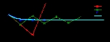
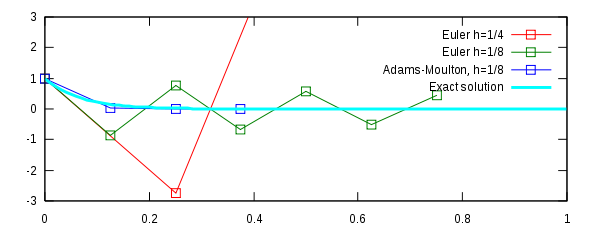
The exact solution (shown in cyan) is with
with  as
as 
We seek a numerical solution that exhibits the same behavior.
The figure (right) illustrates the numerical issues for various numerical integrators applied on the equation.
One of the most prominent examples of the stiff ODEs is a system that describes the chemical reaction of Robertson:
If one treats this system on a short interval, e.g. there is no problem in numerical integration. However, if the interval is very large (
 say), then many standard codes fail to integrate it correctly.
where and
and  is a constant
  matrix with eigenvalues
  (assumed distinct) and corresponding eigenvectors
  . The general solution of (5) takes the form
Mathematics
Mathematics is the study of quantity, space, structure, and change. Mathematicians seek out patterns and formulate new conjectures. Mathematicians resolve the truth or falsity of conjectures by mathematical proofs, which are arguments sufficient to convince other mathematicians of their validity...
, a stiff equation is a differential equation
Differential equation
A differential equation is a mathematical equation for an unknown function of one or several variables that relates the values of the function itself and its derivatives of various orders...
for which certain numerical methods
Numerical ordinary differential equations
Numerical ordinary differential equations is the part of numerical analysis which studies the numerical solution of ordinary differential equations...
for solving the equation are numerically unstable
Numerical stability
In the mathematical subfield of numerical analysis, numerical stability is a desirable property of numerical algorithms. The precise definition of stability depends on the context, but it is related to the accuracy of the algorithm....
, unless the step size is taken to be extremely small. It has proved difficult to formulate a precise definition of stiffness, but the main idea is that the equation includes some terms that can lead to rapid variation in the solution. Solving stiff equations can be a very long and hard process.
When integrating a differential equation numerically, one would expect the requisite step size to be relatively small in a region where the solution curve displays much variation and to be relatively large where the solution curve straightens out to approach a line with slope nearly zero. For some problems this is not the case. Sometimes the step size is forced down to an unacceptably small level in a region where the solution curve is very smooth. The phenomenon being exhibited here is known as stiffness. In some cases we may have two different problems with the same solution, yet problem one is not stiff and problem two is stiff. Clearly the phenomenon cannot be a property of the exact solution, since this is the same for both problems, and must be a property of the differential system itself. It is thus appropriate to speak of stiff systems.
Motivating example
Initial value problem
In mathematics, in the field of differential equations, an initial value problem is an ordinary differential equation together with a specified value, called the initial condition, of the unknown function at a given point in the domain of the solution...
The exact solution (shown in cyan) is
with as We seek a numerical solution that exhibits the same behavior.
The figure (right) illustrates the numerical issues for various numerical integrators applied on the equation.
- Euler's method with a step size of
 oscillates wildly and quickly exits the range of the graph (shown in red).
- Euler's method with half the step size,
 , produces a solution within the graph boundaries, but oscillates about zero (shown in green).
- The trapezoidal method (i.e., the two-stage Adams–Moulton methodMultistep methodLinear multistep methods are used for the numerical solution of ordinary differential equations. Conceptually, a numerical method starts from an initial point and then takes a short step forward in time to find the next solution point. The process continues with subsequent steps to map out the...
) is given by
Applying this method instead of Euler's method gives a much better result (blue). the numerical results decrease monotonically to zero, just as the exact solution does.
One of the most prominent examples of the stiff ODEs is a system that describes the chemical reaction of Robertson:


If one treats this system on a short interval, e.g.
there is no problem in numerical integration. However, if the interval is very large ( say), then many standard codes fail to integrate it correctly.Stiffness ratio
Consider the linear constant coefficient inhomogeneous system
where
and is a constant matrix with eigenvalues (assumed distinct) and corresponding eigenvectors . The general solution of (5) takes the form-

where the κt are arbitrary constants and is a particular integral. Now let us suppose that
-

which implies that each of the terms

as , so that the solution
approaches asymptotically as
  ;
;
the term will decay monotonically if λt is real and sinusoidally if λt is complex.
Interpreting x to be time (as it often is in physical problems)
it is appropriate to call
 the
the
transient solution and the steady-state solution.
If is large, then the corresponding
term will decay quickly as
x increases and is thus called a fast transient; if
 is small, the corresponding term
 decays slowly and is
called a slow transient. Let be defined by
-

so that is the fastest
transient and the
the
slowest. We now define the stiffness ratio as
-

Characterization of stiffness
In this section we consider various aspects of the phenomenon of stiffness. 'Phenomenon' is probably a more appropriate word than 'property', since the latter rather implies that stiffness can be defined in precise mathematical terms; it turns out not to be possible to do this in a satisfactory manner, even for the restricted class of linear constant coefficient systems. We shall also see several qualitative statements that can be (and mostly have been) made in an attempt to encapsulate the notion of stiffness, and state what is probably the most satisfactory of these as a 'definition' of stiffness.
J. D. Lambert defines stiffness as follows:
If a numerical method
Numerical analysisNumerical analysis is the study of algorithms that use numerical approximation for the problems of mathematical analysis ....
with a finite region of absolute stabilityNumerical stabilityIn the mathematical subfield of numerical analysis, numerical stability is a desirable property of numerical algorithms. The precise definition of stability depends on the context, but it is related to the accuracy of the algorithm....
, applied to a system with any initial conditionsInitial value problemIn mathematics, in the field of differential equations, an initial value problem is an ordinary differential equation together with a specified value, called the initial condition, of the unknown function at a given point in the domain of the solution...
, is forced to use in a certain interval of integration a steplength which is excessively small in relation to the smoothness of the exact solution in that interval, then the system is said to be stiff in that interval.
There are other characteristics which are exhibited by many examples of stiff problems, but for each there are counterexamples, so these characteristics do not make good definitions of stiffness. Nonetheless, definitions based upon these characteristics are in common use by some authors and are good clues as to the presence of stiffness. Lambert refers to these as 'statements' rather than definitions, for the aforementioned reasons. A few of these are:- A linear constant coefficient system is stiff if all of its eigenvalues have negative real part and the stiffness ratio is large.
- Stiffness occurs when stability requirements, rather than those of accuracy, constrain the steplength.
- Stiffness occurs when some components of the solution decay much more rapidly than others.
Etymology
The origin of the term 'stiffness' seems to be somewhat of a mystery. According to J. O. Hirschfelder, the term 'stiff' is used because such systems correspond to tight coupling between the driver and driven in servomechanismsServomechanismthumb|right|200px|Industrial servomotorThe grey/green cylinder is the [[Brush |brush-type]] [[DC motor]]. The black section at the bottom contains the [[Epicyclic gearing|planetary]] [[Reduction drive|reduction gear]], and the black object on top of the motor is the optical [[rotary encoder]] for...
.
According to Richard. L. Burden and J. Douglas Faires,
Significant difficulties can occur when standard numerical techniques
Numerical analysisNumerical analysis is the study of algorithms that use numerical approximation for the problems of mathematical analysis ....
are applied to approximate the solution of a differential equationDifferential equationA differential equation is a mathematical equation for an unknown function of one or several variables that relates the values of the function itself and its derivatives of various orders...
when the exact solution contains terms of the form eλt, where λ is a complex number with negative real part.
...
Problems involving rapidly decaying transient solutions occur naturally in a wide variety of applications, including the study of spring and damping systems, the analysis of control systemsControl systemA control system is a device, or set of devices to manage, command, direct or regulate the behavior of other devices or system.There are two common classes of control systems, with many variations and combinations: logic or sequential controls, and feedback or linear controls...
, and problems in chemical kineticsChemical kineticsChemical kinetics, also known as reaction kinetics, is the study of rates of chemical processes. Chemical kinetics includes investigations of how different experimental conditions can influence the speed of a chemical reaction and yield information about the reaction's mechanism and transition...
. These are all examples of a class of problems called stiff (mathematical stiffness) systems of differential equations, due to their application in analyzing the motion of spring and mass systemsHarmonic oscillatorIn classical mechanics, a harmonic oscillator is a system that, when displaced from its equilibrium position, experiences a restoring force, F, proportional to the displacement, x: \vec F = -k \vec x \, where k is a positive constant....
having large spring constantsHooke's lawIn mechanics, and physics, Hooke's law of elasticity is an approximation that states that the extension of a spring is in direct proportion with the load applied to it. Many materials obey this law as long as the load does not exceed the material's elastic limit. Materials for which Hooke's law...
(physical stiffnessStiffnessStiffness is the resistance of an elastic body to deformation by an applied force along a given degree of freedom when a set of loading points and boundary conditions are prescribed on the elastic body.-Calculations:...
).
For example, the initial value problemInitial value problemIn mathematics, in the field of differential equations, an initial value problem is an ordinary differential equation together with a specified value, called the initial condition, of the unknown function at a given point in the domain of the solution...
-

with m = 1, c = 1001, k = 1000, can be written in the form (5) with n = 2 and-

-

-

and has eigenvalues
 . Both eigenvalues have negative real part and the stiffness ratio is
which is fairly large. System (10) then certainly satisfies statements 1 and 3. Here the spring constant k is large and the damping constant c is even larger. (Note that 'large' is a vague, subjective term, but the larger the above quantities are, the more pronounced will be the effect of stiffness.)
The exact solution to (10) is-

Note that (15) behaves quite nearly as a simple exponential , but the presence of the
  term, even with a small coefficient is enough to make the numerical computation very sensitive to step size. Stable integration of (10) requires a very small step size until well into the smooth part of the solution curve, resulting in an error much smaller than required for accuracy. Thus the system also satisfies statement 2 and Lambert's definition.
A-stability
The behaviour of numerical methods on stiff problems can be analyzed by applying these methods to the test equation with
with  . The solution of this equation is
  . This solution approaches zero as
  when
when  . If the numerical method also exhibits this behaviour, then the method is said to be A-stable. A-stable methods do not exhibit the described instability in the motivating example.
Runge–Kutta methods
Runge–Kutta methods applied to the test equation take the form
  , and, by induction,
  . The function φ is called the stability function. Thus, the condition that
  as
as  is equivalent to
  . This motivates the definition of the region of absolute stability (sometimes referred to simply as stability region), which is the set
  . The method is A-stable if the region of absolute stability contains the set
  , that is, the left half plane.
Example: The Euler and trapezoidal methods
Consider both the Euler and trapezoidal methods above. The Euler method applied to the test equation is
is
Hence, with
with  . The region of absolute stability for this method is thus
  which is the disk depicted on the right. The Euler method is not A-stable.
The motivating example had . The value of z when taking step size
  is
is  , which is outside the stability region. Indeed, the numerical results do not converge to zero. However, with step size
  , we have
  which is just inside the stability region and the numerical results converge to zero, albeit rather slowly.
The trapezoidal method
when applied to the test equation , is
, is
Solving for yields
Thus, the stability function is
and the region of absolute stability is
This region contains the left-half plane, so the trapezoidal method is A-stable. In fact, the stability region is identical to the left-half plane, and thus the numerical solution of converges to zero if and only if the exact solution does. Nevertheless, the trapezoidal method does not have perfect stability: it does damp all decaying components, but rapidly decaying components are damped only very mildly, because
  as
as  . This led to the concept of L-stability: a method is L-stable if it is A-stable and
  as
as  . The trapezoidal method is not L-stable. The implicit Euler method is an example of an L-stable method.
General theory
The stability function of a Runge–Kutta method with coefficients A and b is given by
where e denotes the vector with ones. This is a rational functionRational functionIn mathematics, a rational function is any function which can be written as the ratio of two polynomial functions. Neither the coefficients of the polynomials nor the values taken by the function are necessarily rational.-Definitions:...
(one polynomialPolynomialIn mathematics, a polynomial is an expression of finite length constructed from variables and constants, using only the operations of addition, subtraction, multiplication, and non-negative integer exponents...
divided by another).
Explicit Runge–Kutta methods have a strictly lower triangularTriangular matrixIn the mathematical discipline of linear algebra, a triangular matrix is a special kind of square matrix where either all the entries below or all the entries above the main diagonal are zero...
coefficient matrix A and thus, their stability function is a polynomial. It follows that explicit Runge–Kutta methods cannot be A-stable.
The stability function of implicit Runge–Kutta methods is often analyzed using order stars. The order star for a method with stability function is defined to be the set
  . A method is A-stable if and only if its stability function has no poles in the left-hand plane and its order star contains no purely imaginary numbers.
Multistep methods
Linear multistep methodMultistep methodLinear multistep methods are used for the numerical solution of ordinary differential equations. Conceptually, a numerical method starts from an initial point and then takes a short step forward in time to find the next solution point. The process continues with subsequent steps to map out the...
s have the form
Applied to the test equation, they become
which can be simplified to
where . This is a linear recurrence relationRecurrence relationIn mathematics, a recurrence relation is an equation that recursively defines a sequence, once one or more initial terms are given: each further term of the sequence is defined as a function of the preceding terms....
. The method is A-stable if all solutions of the recurrence relation converge to zero when Re z < 0. The characteristic polynomial is
All solutions converge to zero for a given value of if all solutions
  of
of  lie in the unit circle..
The region of absolute stability for a multistep method of the above form is then the set of all for which all
  such that
  satisfy
  . Again, if this set contains the left-half plane, the multi-step method is said to be A-stable.
Example: The second-order Adams–Bashforth method
Let us determine the region of absolute stability for the two-step Adams–Bashforth method
The characteristic polynomial is
which has roots
thus the region of absolute stability is
This region is shown on the right. It does not include all the left half-plane (in fact it only includes the real axis between and
and  ) so the Adams–Bashforth method is not A-stable.
General theory
Explicit multistep methods can never be A-stable, just like explicit Runge–Kutta methods. Implicit multistep methods can only be A-stable if their order is at most 2. The latter result is known as the second DahlquistGermund DahlquistGermund Dahlquist was a Swedish mathematician known primarily for his early contributions to the theory of numerical analysis as applied to differential equations....
barrier; it restricts the usefulness of linear multistep methods for stiff equations. An example of a second-order A-stable method is the trapezoidal rule mentioned above, which can also be considered as a linear multistep method.
External links
-
-
-
-
-
-
-
-


