Simple linear regression
Encyclopedia

Statistics
Statistics is the study of the collection, organization, analysis, and interpretation of data. It deals with all aspects of this, including the planning of data collection in terms of the design of surveys and experiments....
, simple linear regression is the least squares
Ordinary least squares
In statistics, ordinary least squares or linear least squares is a method for estimating the unknown parameters in a linear regression model. This method minimizes the sum of squared vertical distances between the observed responses in the dataset and the responses predicted by the linear...
estimator of a linear regression model with a single explanatory variable
Covariate
In statistics, a covariate is a variable that is possibly predictive of the outcome under study. A covariate may be of direct interest or it may be a confounding or interacting variable....
. In other words, simple linear regression fits a straight line through the set of n points in such a way that makes the sum of squared residuals
Errors and residuals in statistics
In statistics and optimization, statistical errors and residuals are two closely related and easily confused measures of the deviation of a sample from its "theoretical value"...
of the model (that is, vertical distances between the points of the data set and the fitted line) as small as possible.
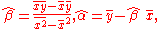
The adjective simple refers to the fact that this regression is one of the simplest in statistics. The fitted line has the slope equal to the correlation between y and x corrected by the ratio of standard deviations of these variables. The intercept of the fitted line is such that it passes through the center of mass (x, y) of the data points.
Other regression methods besides the simple ordinary least squares
Ordinary least squares
In statistics, ordinary least squares or linear least squares is a method for estimating the unknown parameters in a linear regression model. This method minimizes the sum of squared vertical distances between the observed responses in the dataset and the responses predicted by the linear...
(OLS) also exist (see linear regression model). In particular, when one wants to do regression by eye, people usually tend to draw a slightly steeper line, closer to the one produced by the total least squares
Deming regression
In statistics, Deming regression, named after W. Edwards Deming, is an errors-in-variables model which tries to find the line of best fit for a two-dimensional dataset...
method. This occurs because it is more natural for one's mind to consider the orthogonal distances from the observations to the regression line, rather than the vertical ones as OLS method does.
Fitting the regression line
Suppose there are n data points {yi, xi}, where i = 1, 2, …, n. The goal is to find the equation of the straight line
which would provide a "best" fit for the data points. Here the "best" will be understood as in the least-squares
Ordinary least squares
In statistics, ordinary least squares or linear least squares is a method for estimating the unknown parameters in a linear regression model. This method minimizes the sum of squared vertical distances between the observed responses in the dataset and the responses predicted by the linear...
approach: such a line that minimizes the sum of squared residuals of the linear regression model. In other words, numbers α and β solve the following minimization problem:

By using either calculus
Calculus
Calculus is a branch of mathematics focused on limits, functions, derivatives, integrals, and infinite series. This subject constitutes a major part of modern mathematics education. It has two major branches, differential calculus and integral calculus, which are related by the fundamental theorem...
, the geometry of inner product space
Inner product space
In mathematics, an inner product space is a vector space with an additional structure called an inner product. This additional structure associates each pair of vectors in the space with a scalar quantity known as the inner product of the vectors...
s or simply expanding to get a quadratic in α and β, it can be shown that the values of α and β that minimize the objective function Q are
-
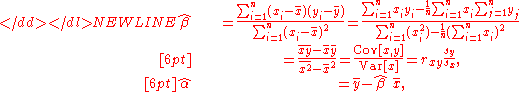
where rxy is the sample correlation coefficient between x and y, sx is the standard deviationStandard deviationStandard deviation is a widely used measure of variability or diversity used in statistics and probability theory. It shows how much variation or "dispersion" there is from the average...
of x, and sy is correspondingly the standard deviation of y. Horizontal bar over a variable means the sample average of that variable. For example:
Substituting the above expressions for and
and  into
into
yields
This shows the role plays in the regression line of standardized data points.
Properties
- The line goes through the "center of mass" point (x, y).
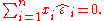
- The sum of the residuals is equal to zero, if the model includes a constant:

- The linear combination of the residuals, in which the coefficients are the x-values, is equal to zero:
- The estimators
 and
and  are unbiased. This requires that we interpret the estimators as random variables and so we have to assume that, for each value of x, the corresponding value of y is generated as a mean response α + βx plus an additional random variable ε called the error term. This error term has to be equal to zero on average, for each value of x. Under such interpretation, the least-squares estimators
  and
and  will themselves be random variables, and they will unbiasedly estimate the "true values" α and β.
Linear regression without the intercept term
Sometimes, people consider a simple linear regression model without the intercept term: y = βx. In such a case, the OLS estimator for β simplifies to .
.
Linear regression with non-uniform errors
If the have independent, non-uniform variances
  , then the function Q above becomes
However, the OLS estimators for α and β are still given by the same equations as above,
except with the averages computed as weighted meansWeighted meanThe weighted mean is similar to an arithmetic mean , where instead of each of the data points contributing equally to the final average, some data points contribute more than others...
of the appropriate variable combinations.
Total least squares method
The above equations assume that {xi} data are known exactly whereas {yi} data have random distribution. In case that both {xi} and {yi} are random we can minimize the orthogonal distances from the observations to the regression line (total least squares method). Here we will show equation for simple linear regression model without the intercept term y = βx under the assumption that x and y have equal variances. For general case please see Deming regressionDeming regressionIn statistics, Deming regression, named after W. Edwards Deming, is an errors-in-variables model which tries to find the line of best fit for a two-dimensional dataset...
.
The orthogonal distance from the observation point {yi, xi} to the regression line y = βx is:
 where
where  denotes absolute valueAbsolute valueIn mathematics, the absolute value |a| of a real number a is the numerical value of a without regard to its sign. So, for example, the absolute value of 3 is 3, and the absolute value of -3 is also 3...
.
We will minimize sum of squared distances:
This can be solved by searching for which derivation
  is zero.
This yields the equation
Which has the solution:
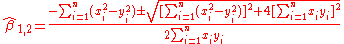
Please note that there are two different solutions (note in the equation above). One solution represent minimum of
  function and the other one maximum of
  function. The corresponding lines are orthogonal to each other. For
  and
and  for all i use + sign to get the slope of the regression line.
It can be shown that if you swap and
and  you will get slope
  . This is not the case for simple linear regression without the intercept term which is using ordinary least squaresOrdinary least squaresIn statistics, ordinary least squares or linear least squares is a method for estimating the unknown parameters in a linear regression model. This method minimizes the sum of squared vertical distances between the observed responses in the dataset and the responses predicted by the linear...
method.
Confidence intervals
The formulas given in the previous section allow one to calculate the point estimates of α and β — that is, the coefficients of the regression line for the given set of data. However, those formulas do not tell us how precise the estimates are. That is, how much the estimators and
and  can deviate from the "true" values of α and β. The latter question is answered by the confidence intervals for the regression coefficients.
In order to construct the confidence intervals usually one of the two possible assumptions is made: either that the errors in the regression are normally distributed (the so-called classic regression assumption), or that the number of observations n is sufficiently large so that the actual distribution of the estimators can be approximated using the Central Limit TheoremCentral limit theoremIn probability theory, the central limit theorem states conditions under which the mean of a sufficiently large number of independent random variables, each with finite mean and variance, will be approximately normally distributed. The central limit theorem has a number of variants. In its common...
.
Normality assumption
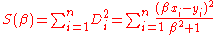
Under the first assumption above, that of the normality of the error terms, the estimator of the slope coefficient will itself be normally distributed with mean β and variance where is the variance of the error terms. At the same time the sum of squared residuals Q is distributed proportionally to χ2 with (n−2) degrees of freedom, and independently from This allows us to construct a t-statistic
-
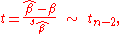 where
where 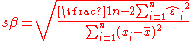
which has a Student's t-distribution with (n−2) degrees of freedom. Here sβ is the standard deviation of the estimator
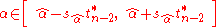
Using this t-statistic we can construct a confidence interval for β:-
 at confidence level (1−γ),
where is the (1−γ/2)-th quantile of the tn–2 distribution. For example, if γ = 0.05 then the confidence level is 95%.
Similarly, the confidence interval for the intercept coefficient α is given by-
 at confidence level (1−γ),
where-

The confidence intervals for α and β give us the general idea where these regression coefficients are most likely to be. For example in the "Okun's law" regression shown at the beginning of the article the point estimates are and The 95% confidence intervals for these estimates are-
 with 95% confidence.
In order to represent this information graphically, in the form of the confidence bands around the regression line, one has to proceed carefully and account for the joint distribution of the estimators. It can be shown that at confidence level (1−γ) the confidence band has hyperbolic form given by the equation-

Asymptotic assumption
The alternative second assumption states that when the number of points in the dataset is "large enough", the Law of large numbersLaw of large numbersIn probability theory, the law of large numbers is a theorem that describes the result of performing the same experiment a large number of times...
and the Central limit theoremCentral limit theoremIn probability theory, the central limit theorem states conditions under which the mean of a sufficiently large number of independent random variables, each with finite mean and variance, will be approximately normally distributed. The central limit theorem has a number of variants. In its common...
become applicable, and then the distribution of the estimators is approximately normal. Under this assumption all formulas derived in the previous section remain valid, with the only exception that the quantile t*n−2 of student-t distribution is replaced with the quantile q* of the standard normal distribution. Occasionally the fraction is replaced with . When n is large such change does not alter the results considerably.
Numerical example
As an example we shall consider the data set from the Ordinary least squaresOrdinary least squaresIn statistics, ordinary least squares or linear least squares is a method for estimating the unknown parameters in a linear regression model. This method minimizes the sum of squared vertical distances between the observed responses in the dataset and the responses predicted by the linear...
article. This data set gives average weights for humans as a function of their height in the population of American women of age 30–39. Although the OLSOrdinary least squaresIn statistics, ordinary least squares or linear least squares is a method for estimating the unknown parameters in a linear regression model. This method minimizes the sum of squared vertical distances between the observed responses in the dataset and the responses predicted by the linear...
article argues that it would be more appropriate to run a quadratic regression for this data, we will not do so and fit the simple linear regression instead.
xi 1.47 1.50 1.52 1.55 1.57 1.60 1.63 1.65 1.68 1.70 1.73 1.75 1.78 1.80 1.83 Height (m) yi 52.21 53.12 54.48 55.84 57.20 58.57 59.93 61.29 63.11 64.47 66.28 68.10 69.92 72.19 74.46 Mass (kg)
There are n = 15 points in this data set, and we start by calculating the following five sums:-

These quantities can be used to calculate the estimates of the regression coefficients, and their standard errors.-
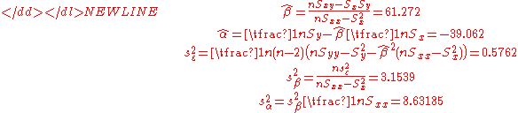
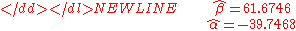
The 0.975 quantile of Student's t-distribution with 13 degrees of freedom is t*13 = 2.1604, and thus confidence intervals for α and β are-

Beware
This example also demonstrates that sophisticated calculations will not overcome the use of badly prepared data. The heights were originally given in inches, and have been converted to the nearest centimetre. Since the conversion factor is one inch to 2.54cm, this is not a correct conversion. The original inches can be recovered by Round(x/0.0254) and then re-converted to metric: if this is done, the results become-
Thus a seemingly small variation in the data has a real effect.
See also
- Proofs involving ordinary least squares — derivation of all formulas used in this article in general multidimensional case;
- Deming regressionDeming regressionIn statistics, Deming regression, named after W. Edwards Deming, is an errors-in-variables model which tries to find the line of best fit for a two-dimensional dataset...
— orthogonal simple linear regression. - Linear segmented regressionSegmented regressionSegmented regression is a method in regression analysis in which the independent variable is partitioned into intervals and a separate line segment is fit to each interval. Segmented or piecewise regression analysis can also be performed on multivariate data by partitioning the various independent...
-
-
-
-
-
-