Rössler attractor - AbsoluteAstronomy.com

The Rössler attractor is the attractor

Attractor

An attractor is a set towards which a dynamical system evolves over time. That is, points that get close enough to the attractor remain close even if slightly disturbed...

for the Rössler system, a system of three non-linear ordinary differential equation

Ordinary differential equation

In mathematics, an ordinary differential equation is a relation that contains functions of only one independent variable, and one or more of their derivatives with respect to that variable....

s. These differential equations define a continuous-time dynamical system that exhibits chaotic

Chaos theory

Chaos theory is a field of study in mathematics, with applications in several disciplines including physics, economics, biology, and philosophy. Chaos theory studies the behavior of dynamical systems that are highly sensitive to initial conditions, an effect which is popularly referred to as the...

dynamics associated with the fractal properties of the attractor. Some properties of the Rössler system can be deduced via linear methods such as eigenvectors, but the main features of the system require non-linear methods such as Poincaré map

Poincaré map

In mathematics, particularly in dynamical systems, a first recurrence map or Poincaré map, named after Henri Poincaré, is the intersection of a periodic orbit in the state space of a continuous dynamical system with a certain lower dimensional subspace, called the Poincaré section, transversal to...

s and bifurcation diagram

Bifurcation diagram

In mathematics, particularly in dynamical systems, a bifurcation diagram shows the possible long-term values of a system as a function of a bifurcation parameter in the system...

s. The original Rössler paper says the Rössler attractor was intended to behave similarly to the Lorenz attractor

Lorenz attractor

The Lorenz attractor, named for Edward N. Lorenz, is an example of a non-linear dynamic system corresponding to the long-term behavior of the Lorenz oscillator. The Lorenz oscillator is a 3-dimensional dynamical system that exhibits chaotic flow, noted for its lemniscate shape...

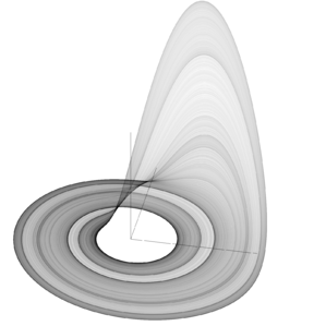
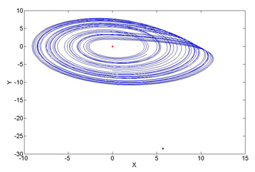
, but also be easier to analyze qualitatively. An orbit within the attractor follows an outward spiral close to the

plane around an unstable fixed point. Once the graph spirals out enough, a second fixed point influences the graph, causing a rise and twist in the

-dimension. In the time domain, it becomes apparent that although each variable is oscillating within a fixed range of values, the oscillations are chaotic. This attractor has some similarities to the Lorenz attractor, but is simpler and has only one manifold

Manifold

In mathematics , a manifold is a topological space that on a small enough scale resembles the Euclidean space of a specific dimension, called the dimension of the manifold....

. Otto Rössler

Otto Rössler

Otto E. Rössler is a German biochemist and is notable for his work on chaos theory and his theoretical equation known as the Rössler attractor.-Biography:...

designed the Rössler attractor in 1976, but the originally theoretical equations were later found to be useful in modeling equilibrium in chemical reactions. The defining equations are:

Rössler studied the chaotic attractor with

, and

, though properties of

, and

have been more commonly used since.

An analysis

Some of the Rössler attractor's elegance is due to two of its equations being linear; setting

, allows examination of the behavior on the

plane

The stability in the

plane can then be found by calculating the eigenvalues of the Jacobian

Jacobian

In vector calculus, the Jacobian matrix is the matrix of all first-order partial derivatives of a vector- or scalar-valued function with respect to another vector. Suppose F : Rn → Rm is a function from Euclidean n-space to Euclidean m-space...

, which are

. From this, we can see that when

, the eigenvalues are complex and both have a positive real component, making the origin unstable with an outwards spiral on the

plane. Now consider the

plane behavior within the context of this range for

. So long as

is smaller than

, the

term will keep the orbit close to the

plane. As the orbit approaches

greater than

, the

-values begin to climb. As

climbs, though, the

in the equation for

stops the growth in

Fixed points

In order to find the fixed points, the three Rössler equations are set to zero and the (

) coordinates of each fixed point were determined by solving the resulting equations. This yields the general equations of each of the fixed point coordinates:

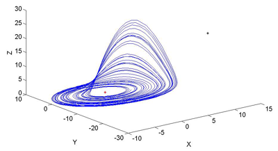
Which in turn can be used to show the actual fixed points for a given set of parameter values:

As shown in the general plots of the Rössler Attractor above, one of these fixed points resides in the center of the attractor loop and the other lies comparatively removed from the attractor.

Eigenvalues and eigenvectors

The stability of each of these fixed points can be analyzed by determining their respective eigenvalues and eigenvectors. Beginning with the Jacobian:

the eigenvalues can be determined by solving the following cubic:

For the centrally located fixed point, Rössler’s original parameter values of a=0.2, b=0.2, and c=5.7 yield eigenvalues of:

(Using Mathematica 7)

The magnitude of a negative eigenvalue characterizes the level of attraction along the corresponding eigenvector. Similarly the magnitude of a positive eigenvalue characterizes the level of repulsion along the corresponding eigenvector.

The eigenvectors corresponding to these eigenvalues are:

These eigenvectors have several interesting implications. First, the two eigenvalue/eigenvector pairs (

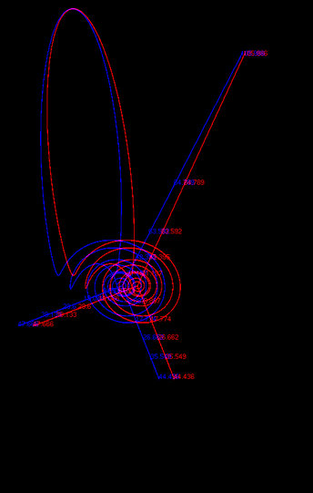
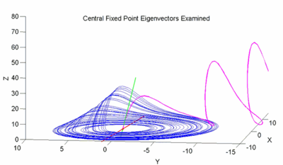
and

) are responsible for the steady outward slide that occurs in the main disk of the attractor. The last eigenvalue/eigenvector pair is attracting along an axis that runs through the center of the manifold and accounts for the z motion that occurs within the attractor. This effect is roughly demonstrated with the figure below.

The figure examines the central fixed point eigenvectors. The blue line corresponds to the standard Rössler attractor generated with

, and

. The red dot in the center of this attractor is

. The red line intersecting that fixed point is an illustration of the repulsing plane generated by

and

. The green line is an illustration of the attracting

. The magenta line is generated by stepping backwards through time from a point on the attracting eigenvector which is slightly above

– it illustrates the behavior of points that become completely dominated by that vector. Note that the magenta line nearly touches the plane of the attractor before being pulled upwards into the fixed point; this suggests that the general appearance and behavior of the Rössler attractor is largely a product of the interaction between the attracting

and the repelling

and

plane. Specifically it implies that a sequence generated from the Rössler equations will begin to loop around

, start being pulled upwards into the

vector, creating the upward arm of a curve that bends slightly inward toward the vector before being pushed outward again as it is pulled back towards the repelling plane.

For the outlier fixed point, Rössler’s original parameter values of

, and

yield eigenvalues of:

The eigenvectors corresponding to these eigenvalues are:

Although these eigenvalues and eigenvectors exist in the Rössler attractor, their influence is confined to iterations of the Rössler system whose initial conditions are in the general vicinity of this outlier fixed point. Except in those cases where the initial conditions lie on the attracting plane generated by

and

, this influence effectively involves pushing the resulting system towards the general Rössler attractor. As the resulting sequence approaches the central fixed point and the attractor itself, the influence of this distant fixed point (and its eigenvectors) will wane.

Poincaré map

The Poincaré map

Poincaré map

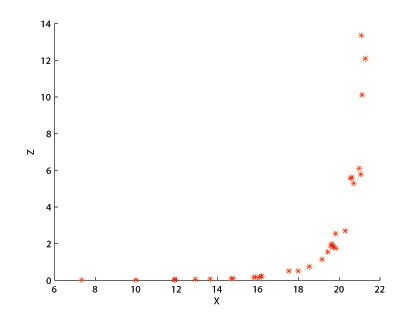
is constructed by plotting the value of the function every time it passes through a set plane in a specific direction. An example would be plotting the

value every time it passes through the

plane where

is changing from negative to positive, commonly done when studying the Lorenz attractor. In the case of the Rössler attractor, the

plane is uninteresting, as the map always crosses the

plane at

due to the nature of the Rössler equations. In the

plane for

, the Poincaré map shows the upswing in

values as

increases, as is to be expected due to the upswing and twist section of the Rössler plot. The number of points in this specific Poincaré plot is infinite, but when a different

value is used, the number of points can vary. For example, with a

value of 4, there is only one point on the Poincaré map, because the function yields a periodic orbit of period one, or if the

value is set to 12.8, there would be six points corresponding to a period six orbit.

Mapping local maxima

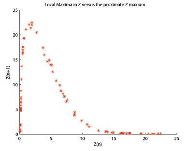
In the original paper on the Lorenz Attractor, Edward Lorenz analyzed the local maxima of

against the immediately preceding local maxima. When visualized, the plot resembled the tent map, implying that similar analysis can be used between the map and attractor. For the Rössler attractor, when the

local maximum is plotted against the next local

maximum,

, the resulting plot
(shown here for

) is unimodal, resembling a skewed Henon map. Knowing that the Rössler attractor can be used to create a pseudo 1-d map, it then follows to use similar analysis methods. The bifurcation diagram is specifically a useful analysis method.

Variation of parameters

Rössler attractor's behavior is largely a factor of the values of its constant parameters

, and

. In general, varying each parameter has a comparable effect by causing the system to converge toward a periodic orbit, fixed point, or escape towards infinity, however the specific ranges and behaviors induced vary substantially for each parameter. Periodic orbits, or "unit cycles," of the Rössler system are defined by the number of loops around the central point that occur before the loops series begins to repeat itself.

Bifurcation diagram

Bifurcation diagram

In mathematics, particularly in dynamical systems, a bifurcation diagram shows the possible long-term values of a system as a function of a bifurcation parameter in the system...

s are a common tool for analyzing the behavior of dynamical system

Dynamical system

A dynamical system is a concept in mathematics where a fixed rule describes the time dependence of a point in a geometrical space. Examples include the mathematical models that describe the swinging of a clock pendulum, the flow of water in a pipe, and the number of fish each springtime in a...

s, of which the Rössler attractor is one. They are created by running the equations of the system, holding all but one of the variables constant and varying the last one. Then, a graph.is plotted of the points that a particular value for the changed variable visits after transient factors have been neutralised. Chaotic regions are indicated by filled-in regions of the plot.

Varying a

Here,

is fixed at 0.2,

is fixed at 5.7 and

changes. Numerical examination of the attractor's behavior over changing

suggests it has a disproportional influence over the attractor's behavior. The results of the analysis are:

: Converges to the centrally located fixed point
: Unit cycle of period 1
: Standard parameter value selected by Rössler, chaotic
: Chaotic attractor, significantly more Möbius strip
Möbius strip
The Möbius strip or Möbius band is a surface with only one side and only one boundary component. The Möbius strip has the mathematical property of being non-orientable. It can be realized as a ruled surface...

-like (folding over itself).
: Similar to .3, but increasingly chaotic
: Similar to .35, but increasingly chaotic.

Varying b

Here,

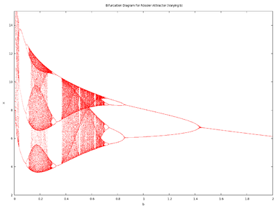
is fixed at 0.2,

is fixed at 5.7 and

changes. As shown in the accompanying diagram, as

approaches 0 the attractor approaches infinity (note the upswing for very small values of

. Comparative to the other parameters, varying

generates a greater range when period-3 and period-6 orbits will occur. In contrast to

and

, higher values of

converge to period-1, not to a chaotic state.

Varying c

Here,

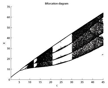
and

changes. The bifurcation diagram

Bifurcation diagram

In mathematics, particularly in dynamical systems, a bifurcation diagram shows the possible long-term values of a system as a function of a bifurcation parameter in the system...

reveals that low values of

are periodic, but quickly become chaotic as

increases. This pattern repeats itself as

increases – there are sections of periodicity interspersed with periods of chaos, and the trend is towards higher-period orbits as

increases. For example, the period one orbit only appears for values of

around 4 and is never found again in the bifurcation diagram. The same phenomenon is seen with period three; until

, period three orbits can be found, but thereafter, they do not appear.

A graphical illustration of the changing attractor over a range of

values illustrates the general behavior seen for all of these parameter analyses – the frequent transitions between periodicity and aperiodicity.

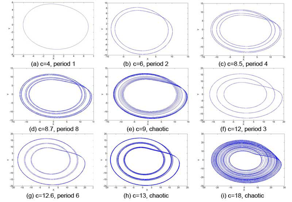
The above set of images illustrates the variations in the post-transient Rössler system as

is varied over a range of values. These images were generated with

, period-1 orbit.
, period-2 orbit.
, period-4 orbit.
, period-8 orbit.
, sparse chaotic attractor.
, period-3 orbit.
, period-6 orbit.
, sparse chaotic attractor.
, filled-in chaotic attractor.

Links to other topics

The banding evident in the Rössler attractor is similar to a Cantor set

Cantor set

In mathematics, the Cantor set is a set of points lying on a single line segment that has a number of remarkable and deep properties. It was discovered in 1875 by Henry John Stephen Smith and introduced by German mathematician Georg Cantor in 1883....

rotated about its midpoint. Additionally, the half-twist in the Rössler attractor makes it similar to a Möbius strip

Möbius strip

The Möbius strip or Möbius band is a surface with only one side and only one boundary component. The Möbius strip has the mathematical property of being non-orientable. It can be realized as a ruled surface...

External links

The source of this article is wikipedia, the free encyclopedia. The text of this article is licensed under the GFDL.

An analysis

Fixed points

Eigenvalues and eigenvectors

Poincaré map

Mapping local maxima

Variation of parameters

Varying a

Varying b

Varying c

Links to other topics

See also

External links