
MUSCL scheme
Encyclopedia
In the study of partial differential equation
s, the MUSCL scheme is a finite volume method
that can provide highly accurate numerical solutions for a given system, even in cases where the solutions exhibit shocks, discontinuities, or large gradients. MUSCL stands for Monotone Upstream-centered Schemes for Conservation Laws, and the term was introduced in a seminal paper by Bram van Leer
(van Leer, 1979). In this paper he constructed the first high-order, total variation diminishing
(TVD) scheme where he obtained second order spatial accuracy.
The idea is to replace the piecewise constant approximation of Godunov's scheme
by reconstructed states, derived from cell-averaged states obtained from the previous time-step. For each cell, slope limited, reconstructed left and right states are obtained and used to calculate fluxes at the cell boundaries (edges). These fluxes can, in turn, be used as input to a Riemann solver
, following which the solutions are averaged and used to advance the solution in time. Alternatively, the fluxes can be used in Riemann-solver-free schemes, such as the Kurganov and Tadmor scheme outlined below.
 We will consider the fundamentals of the MUSCL scheme by considering the following simple first-order, scalar, 1D system, which is assumed to have a wave propagating in the positive direction,

Where represents a state variable and
  represents a flux
variable.
The basic scheme of Godunov uses piecewise constant approximations for each cell, and results in a first-order upwind discretisation of the above problem with cell centres indexed as . A semi-discrete scheme can be defined as follows,
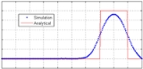
This basic scheme is not able to handle shocks or sharp discontinuities as they tend to become smeared. An example of this effect is shown in the diagram opposite, which illustrates a 1D advective equation with a step wave propagating to the right. The simulation was carried out with a mesh of 200 cells and used a 4th order Runge–Kutta time integrator (RK4).
To provide higher resolution of discontinuities, Godunov's scheme can be extended to use piecewise linear approximations of each cell, which results in a central difference scheme that is second-order accurate in space. The piecewise linear approximations are obtained from
Thus, evaluating fluxes at the cell edges we get the following semi-discrete scheme
 where
where  and
and  are the piecewise approximate values of cell edge variables, i.e.
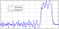
Although the above second-order scheme provides greater accuracy for smooth solutions, it is not a total variation diminishing
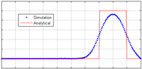
(TVD) scheme and introduces spurious oscillations into the solution where discontinuities or shocks are present. An example of this effect is shown in the diagram opposite, which illustrates a 1D advective equation , with a step wave propagating to the right. This loss of accuracy is to be expected due to Godunov's theorem
. The simulation was carried out with a mesh of 200 cells and used RK4 for time integration.
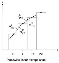 MUSCL based numerical schemes extend the idea of using a linear piecewise approximation to each cell by using slope limited left and right extrapolated states. This results in the following high resolution, TVD discretisation scheme,
Which, alternatively, can be written in the more succinct form,
The numerical fluxes correspond to a nonlinear combination of first and second-order approximations to the continuous flux function.
The symbols and
and  represent scheme dependent functions (of the limited extrapolated cell edge variables), i.e.
and


The function is a limiter function that limits the slope of the piecewise approximations to ensure the solution is TVD, thereby avoiding the spurious oscillations that would otherwise occur around discontinuities or shocks - see Flux limiter
section. The limiter is equal to zero when and is equal to unity when
  . Thus, the accuracy of a TVD discretization degrades to first order at local extrema, but tends to second order over smooth parts of the domain.
The algorithm is straight forward to implement. Once a suitable scheme for has been chosen, such as the Kurganov and Tadmor scheme (see below), the solution can proceed using standard numerical integration techniques.
and vector problems , and can be viewed as a modification to the Lax-Friedrichs (LxF) scheme. The algorithm is based upon central differences
with comparable performance to Riemann type solvers when used to obtain solutions for PDE's describing systems that exhibit high-gradient phenomena.
The KT scheme extends the NT scheme and has a smaller amount of numerical viscosity than the original NT scheme. It also has the added advantage that it can be implemented as either a fully discrete or semi-discrete scheme. Here we consider the semi-discrete scheme.
The calculation is shown below:
Partial differential equation
In mathematics, partial differential equations are a type of differential equation, i.e., a relation involving an unknown function of several independent variables and their partial derivatives with respect to those variables...
s, the MUSCL scheme is a finite volume method
Finite volume method
The finite volume method is a method for representing and evaluating partial differential equations in the form of algebraic equations [LeVeque, 2002; Toro, 1999]....
that can provide highly accurate numerical solutions for a given system, even in cases where the solutions exhibit shocks, discontinuities, or large gradients. MUSCL stands for Monotone Upstream-centered Schemes for Conservation Laws, and the term was introduced in a seminal paper by Bram van Leer
Bram van Leer
Bram van Leer is the Arthur B. Modine Professor of aerospace engineering at the University of Michigan, in Ann Arbor. He specialises in Computational fluid dynamics , fluid dynamics, and numerical analysis where he has made substantial contributions.-Research work:Professor van Leer developed...
(van Leer, 1979). In this paper he constructed the first high-order, total variation diminishing
Total variation diminishing
In numerical methods, total variation diminishing is a property of certain discretization schemes used to solve hyperbolic partial differential equations...
(TVD) scheme where he obtained second order spatial accuracy.
The idea is to replace the piecewise constant approximation of Godunov's scheme
Godunov's scheme
In numerical analysis and computational fluid dynamics, Godunov's scheme is a conservative numerical scheme, suggested by S. K. Godunov in 1959, for solving partial differential equations...
by reconstructed states, derived from cell-averaged states obtained from the previous time-step. For each cell, slope limited, reconstructed left and right states are obtained and used to calculate fluxes at the cell boundaries (edges). These fluxes can, in turn, be used as input to a Riemann solver
Riemann solver
A Riemann solver is a numerical method used to solve a Riemann problem. They are heavily used in computational fluid dynamics and computational magnetohydrodynamics.-Exact solvers:...
, following which the solutions are averaged and used to advance the solution in time. Alternatively, the fluxes can be used in Riemann-solver-free schemes, such as the Kurganov and Tadmor scheme outlined below.
Linear reconstruction
Where
represents a state variable and represents a fluxFlux
In the various subfields of physics, there exist two common usages of the term flux, both with rigorous mathematical frameworks.* In the study of transport phenomena , flux is defined as flow per unit area, where flow is the movement of some quantity per time...
variable.
The basic scheme of Godunov uses piecewise constant approximations for each cell, and results in a first-order upwind discretisation of the above problem with cell centres indexed as
. A semi-discrete scheme can be defined as follows,This basic scheme is not able to handle shocks or sharp discontinuities as they tend to become smeared. An example of this effect is shown in the diagram opposite, which illustrates a 1D advective equation with a step wave propagating to the right. The simulation was carried out with a mesh of 200 cells and used a 4th order Runge–Kutta time integrator (RK4).
To provide higher resolution of discontinuities, Godunov's scheme can be extended to use piecewise linear approximations of each cell, which results in a central difference scheme that is second-order accurate in space. The piecewise linear approximations are obtained from
Thus, evaluating fluxes at the cell edges we get the following semi-discrete scheme
and are the piecewise approximate values of cell edge variables, i.e.Although the above second-order scheme provides greater accuracy for smooth solutions, it is not a total variation diminishing
Total variation diminishing
In numerical methods, total variation diminishing is a property of certain discretization schemes used to solve hyperbolic partial differential equations...
(TVD) scheme and introduces spurious oscillations into the solution where discontinuities or shocks are present. An example of this effect is shown in the diagram opposite, which illustrates a 1D advective equation
, with a step wave propagating to the right. This loss of accuracy is to be expected due to Godunov's theoremGodunov's theorem
In numerical analysis and computational fluid dynamics, Godunov's theorem — also known as Godunov's order barrier theorem — is a mathematical theorem important in the development of the theory of high resolution schemes for the numerical solution of partial differential equations.The theorem states...
. The simulation was carried out with a mesh of 200 cells and used RK4 for time integration.
Which, alternatively, can be written in the more succinct form,
The numerical fluxes
correspond to a nonlinear combination of first and second-order approximations to the continuous flux function.The symbols
and represent scheme dependent functions (of the limited extrapolated cell edge variables), i.e.and
The function
is a limiter function that limits the slope of the piecewise approximations to ensure the solution is TVD, thereby avoiding the spurious oscillations that would otherwise occur around discontinuities or shocks - see Flux limiterFlux limiter
Flux limiters are used in high resolution schemes – numerical schemes used to solve problems in science and engineering, particularly fluid dynamics, described by partial differential equations...
section. The limiter is equal to zero when
and is equal to unity when . Thus, the accuracy of a TVD discretization degrades to first order at local extrema, but tends to second order over smooth parts of the domain.The algorithm is straight forward to implement. Once a suitable scheme for
has been chosen, such as the Kurganov and Tadmor scheme (see below), the solution can proceed using standard numerical integration techniques.Kurganov and Tadmor central scheme
A precursor to the Kurganov and Tadmor (KT) central scheme, (Kurganov and Tadmor, 2000), is the Nessyahu and Tadmor (NT) central scheme, (Nessyahu and Tadmor, 1990). It is a Riemann-solver-free, second-order, high-resolution scheme that uses MUSCL reconstruction. It is a fully discrete method that is straight forward to implement and can be used on scalarScalar (mathematics)
In linear algebra, real numbers are called scalars and relate to vectors in a vector space through the operation of scalar multiplication, in which a vector can be multiplied by a number to produce another vector....
and vector problems , and can be viewed as a modification to the Lax-Friedrichs (LxF) scheme. The algorithm is based upon central differences
Finite difference
A finite difference is a mathematical expression of the form f − f. If a finite difference is divided by b − a, one gets a difference quotient...
with comparable performance to Riemann type solvers when used to obtain solutions for PDE's describing systems that exhibit high-gradient phenomena.
The KT scheme extends the NT scheme and has a smaller amount of numerical viscosity than the original NT scheme. It also has the added advantage that it can be implemented as either a fully discrete or semi-discrete scheme. Here we consider the semi-discrete scheme.
The calculation is shown below:
-

-

Where the local propagation speed,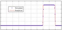
 , is the maximum absolute value of the eigenvalue of the Jacobian of
  over cells
  given by
-

where represents the spectral radiusSpectral radiusIn mathematics, the spectral radius of a square matrix or a bounded linear operator is the supremum among the absolute values of the elements in its spectrum, which is sometimes denoted by ρ.-Matrices:...
of

Beyond these CFLCourant–Friedrichs–Lewy conditionIn mathematics, the Courant–Friedrichs–Lewy condition is a necessary condition for convergence while solving certain partial differential equations numerically by the method of finite differences. It arises when explicit time-marching schemes are used for the numerical solution...
related speeds, no characteristic information is required.
The above flux calculation is sometimes referred to as local Lax-Friedrichs flux or Rusanov flux (Lax, 1954; Rusanov, 1961; Toro, 1999; Kurganov and Tadmor, 2000; Leveque, 2002).
An example of the effectiveness of using a high resolution scheme is shown in the diagram opposite, which illustrates the 1D advective equation , with a step wave propagating to the right. The simulation was carried out on a mesh of 200 cells, using the Kurganov and Tadmor central scheme with Superbee limiterFlux limiterFlux limiters are used in high resolution schemes – numerical schemes used to solve problems in science and engineering, particularly fluid dynamics, described by partial differential equations...
and used RK-4 for time integration. This simulation result contrasts extremely well against the above first-order upwind and second-order central difference results shown above. This scheme also provides good results when applied to sets of equations - see results below for this scheme applied to the Euler equations. However, care has to be taken in choosing an appropriate limiter because, for example, the Superbee limiter can cause unrealistic sharpening for some smooth waves.
The scheme can readily include diffusion terms, if they are present. For example, if the above 1D scalar problem is extended to include a diffusion term, we get
for which Kurganov and Tadmor propose the following central difference approximation,
Where,
Full details of the algorithm (full and semi-discrete versions) and its derivation can be found in the original paper (Kurganov and Tadmor, 2000), along with a number of 1D and 2D examples. Additional information is also available in the earlier related paper by Nessyahu and Tadmor (1990).
Note: This scheme was originally presented by Kurganov and Tadmor as a 2nd order scheme based upon linear extrapolation. A later paper (Kurganov and Levy, 2000) demonstrates that it can also form the basis of a third order scheme. A 1D advective example and an Euler equation example of their scheme, using parabolic reconstruction (3rd order), are shown in the parabolic reconstruction and Euler equation sections below.
Piecewise parabolic reconstruction
It is possible to extend the idea of linear-extrapolation to higher order reconstruction, and an example is shown in the diagram opposite. However, for this case the left and right states are estimated by interpolation of a second-order, upwind biased, difference equation. This results in a parabolic reconstruction scheme that is third-order accurate in space.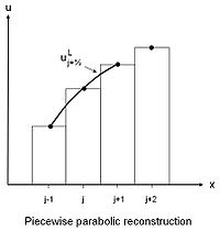
We follow the approach of Kermani (Kermani, et al., 2003), and present a third-order upwind biased scheme, where the symbols and
and  again represent scheme dependent functions (of the limited reconstructed cell edge variables). But for this case they are based upon parabolically reconstructed states, i.e.
and
Where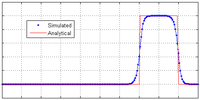
 = 1/3 and,

and the limiter function , is the same as above.
Parabolic reconstruction is straight forward to implement and can be used with the Kurganov and Tadmor scheme in lieu of the linear extrapolation shown above. This has the effect of raising the spatial solution of the KT scheme to 3rd order. It performs well when solving the Euler equations, see below. This increase in spatial order has certain advantages over 2nd order schemes for smooth solutions, however, for shocks it is more dissipative - compare diagram opposite with above solution obtained using the KT algorithm with linear extrapolation and Superbee limiter. This simulation was carried out on a mesh of 200 cells using the same KT algorithm but with parabolic reconstruction. Time integration was by RK-4, and the alternative form of van Albada limiter, , was used to avoid spurious oscillations.
Example: 1D Euler equations
For simplicity we consider the 1D case without heat transfer and without body force. Therefore, in conservation vector form, the general Euler equations reduce to

where
and where is a vector of states and
  is a vector of fluxes.
The equations above represent conservation of mass, momentum, and energy. There are thus three equations and four unknowns, (density)
  (fluid velocity),
  (pressure) and
  (total energy). The total energy is given by,

where represents specific internal energy.
In order to close the system an equation of stateEquation of stateIn physics and thermodynamics, an equation of state is a relation between state variables. More specifically, an equation of state is a thermodynamic equation describing the state of matter under a given set of physical conditions...
is required. One that suits our purpose is

where is equal to the ratio of specific heats
  for the fluid.
We can now proceed, as shown above in the simple 1D example, by obtaining the left and right extrapolated states for each state variable. Thus, for density we obtain
where


Similarly, for momentum , and total energy
  . Velocity
  , is calculated from momentum, and pressure
  , is calculated from the equation of state.
Having obtained the limited extrapolated states, we then proceed to construct the edge fluxes using these values. With the edge fluxes known, we can now construct the semi-discrete scheme, i.e.
The solution can now proceed by integration using standard numerical techniques.
The above illustrates the basic idea of the MUSCL scheme. However, for a practical solution to the Euler equations, a suitable scheme (such as the above KT scheme), also has to be chosen in order to define the function .
.
The diagram opposite shows a 2nd order solution to G A Sod's shock tube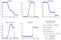 Shock tubeFor the pyrotechnic initiator, see Shock tube detonatorThe shock tube is an instrument used to replicate and direct blast waves at a sensor or a model in order to simulate actual explosions and their effects, usually on a smaller scale...
problem (Sod, 1978) using the above high resolution Kurganov and Tadmor Central Scheme (KT) with Linear Extrapolation and Ospre limiter. This illustrates clearly the effectiveness of the MUSCL approach to solving the Euler equations. The simulation was carried out on a mesh of 200 cells using Matlab code (Wesseling, 2001), adapted to use the KT algorithm and Ospre limiterFlux limiterFlux limiters are used in high resolution schemes – numerical schemes used to solve problems in science and engineering, particularly fluid dynamics, described by partial differential equations...
. Time integration was performed by a 4th order SHK (equivalent performance to RK-4) integrator. The following initial conditions (SISiSi, si, or SI may refer to :- Measurement, mathematics and science :* International System of Units , the modern international standard version of the metric system...
units) were used:
- pressure left = 100000 [Pa];
- pressure right= 10000 [Pa];
- density left = 1.0 [kg/m3];
- density right = 0.125 [kg/m3];
- length = 20 [m];
- velocity left = 0 [m/s];
- velocity right = 0 [m/s];
- duration =0.01 [s];
- lambda = 0.001069 (Δt/Δx).
The diagram opposite shows a 3rd order solution to G A Sod's shock tube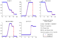 Shock tubeFor the pyrotechnic initiator, see Shock tube detonatorThe shock tube is an instrument used to replicate and direct blast waves at a sensor or a model in order to simulate actual explosions and their effects, usually on a smaller scale...
problem (Sod, 1978) using the above high resolution Kurganov and Tadmor Central Scheme (KT) but with parabolic reconstruction and van Albada limiter. This again illustrates the effectiveness of the MUSCL approach to solving the Euler equations. The simulation was carried out on a mesh of 200 cells using Matlab code (Wesseling, 2001), adapted to use the KT algorithm with Parabolic Extrapolation and van Albada limiterFlux limiterFlux limiters are used in high resolution schemes – numerical schemes used to solve problems in science and engineering, particularly fluid dynamics, described by partial differential equations...
. The alternative form of van Albada limiter, , was used to avoid spurious oscillations. Time integration was performed by a 4th order SHK integrator. The same initial conditions were used.
Various other high resolution schemes have been developed that solve the Euler equations with good accuracy. Examples of such schemes are,
- the Osher scheme, and
- the Liou-Steffen AUSMAUSMAUSM stands for Advection Upstream Splitting Method. It is developed as a numerical inviscid flux function for solving a general system of conservation equations...
(advection upstream splitting method) scheme.
More information on these and other methods can be found in the references below.
See also
- Finite volume methodFinite volume methodThe finite volume method is a method for representing and evaluating partial differential equations in the form of algebraic equations [LeVeque, 2002; Toro, 1999]....
- Flux limiterFlux limiterFlux limiters are used in high resolution schemes – numerical schemes used to solve problems in science and engineering, particularly fluid dynamics, described by partial differential equations...
- Godunov's theoremGodunov's theoremIn numerical analysis and computational fluid dynamics, Godunov's theorem — also known as Godunov's order barrier theorem — is a mathematical theorem important in the development of the theory of high resolution schemes for the numerical solution of partial differential equations.The theorem states...
- High resolution schemeHigh resolution schemeHigh-resolution schemes are used in the numerical solution of partial differential equations where high accuracy is required in the presence of shocks or discontinuities...
- Method of linesMethod of linesThe method of lines is a technique for solving partial differential equations in which all but one dimension is discretized. MOL allows standard, general-purpose methods and software, developed for the numerical integration of ODEs and DAEs, to be used...
- Sergei K. GodunovSergei K. GodunovSergei Konstantinovich Godunov is professor at the Sobolev Institute of Mathematics of the Russian Academy of Sciences in Novosibirsk, Russia....
- Total variation diminishingTotal variation diminishingIn numerical methods, total variation diminishing is a property of certain discretization schemes used to solve hyperbolic partial differential equations...
Further reading
- Hirsch, C. (1990), Numerical Computation of Internal and External Flows, vol 2, Wiley.
- Laney, Culbert B. (1998), Computational Gas Dynamics, Cambridge University Press.
- Tannehill, John C., et al. (1997), Computational Fluid mechanics and Heat Transfer, 2nd Ed., Taylor and Francis.
-
-