Levinson recursion
Encyclopedia
Levinson recursion or Levinson-Durbin recursion is a procedure in linear algebra
to recursively
calculate the solution to an equation involving a Toeplitz matrix
. The algorithm runs in Θ
(n2) time, which is a strong improvement over Gauss-Jordan elimination, which runs in Θ(n3).
Newer algorithms, called asymptotically fast or sometimes superfast Toeplitz algorithms, can solve in Θ(n logpn) for various p (e.g. p = 2, p = 3 ). Levinson recursion remains popular for several reasons; for one, it is relatively easy to understand in comparison; for another, it can be faster than a superfast algorithm for small n (usually n < 256).
The Levinson-Durbin algorithm was proposed first by Norman Levinson
in 1947, improved by J. Durbin in 1960, and subsequently improved to 4n2 and then 3n2 multiplications by W. F. Trench and S. Zohar, respectively.
Other methods to process data include Schur decomposition
and Cholesky decomposition
. In comparison to these, Levinson recursion (particularly Split-Levinson recursion) tends to be faster computationally, but more sensitive to computational inaccuracies like round-off error
s.
The Levinson-Durbin algorithm may be used for any such equation, as long as M is a known Toeplitz matrix
with a nonzero main diagonal. Here is a known vector
, and is an unknown vector of numbers xi yet to be determined.
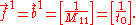
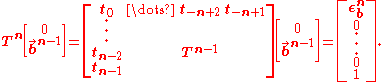
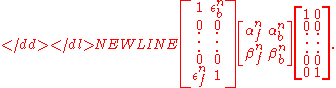
For the sake of this article, êi is a vector made up entirely of zeroes, except for its i'th place, which holds the value one. Its length will be implicitly determined by the surrounding context. The term N refers to the width of the matrix above -- M is an N×N matrix. Finally, in this article, superscripts refer to an inductive index, whereas subscripts denote indices. For example (and definition), in this article, the matrix Tn is an n×n matrix which copies the upper left n×n block from M -- that is, Tnij = Mij.
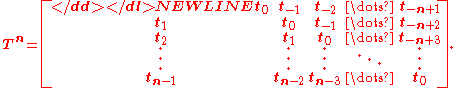
Tn is also a Toeplitz matrix; meaning that it can be written as:
Linear algebra
Linear algebra is a branch of mathematics that studies vector spaces, also called linear spaces, along with linear functions that input one vector and output another. Such functions are called linear maps and can be represented by matrices if a basis is given. Thus matrix theory is often...
to recursively
Recursion
Recursion is the process of repeating items in a self-similar way. For instance, when the surfaces of two mirrors are exactly parallel with each other the nested images that occur are a form of infinite recursion. The term has a variety of meanings specific to a variety of disciplines ranging from...
calculate the solution to an equation involving a Toeplitz matrix
Toeplitz matrix
In linear algebra, a Toeplitz matrix or diagonal-constant matrix, named after Otto Toeplitz, is a matrix in which each descending diagonal from left to right is constant...
. The algorithm runs in Θ
Big O notation
In mathematics, big O notation is used to describe the limiting behavior of a function when the argument tends towards a particular value or infinity, usually in terms of simpler functions. It is a member of a larger family of notations that is called Landau notation, Bachmann-Landau notation, or...
(n2) time, which is a strong improvement over Gauss-Jordan elimination, which runs in Θ(n3).
Newer algorithms, called asymptotically fast or sometimes superfast Toeplitz algorithms, can solve in Θ(n logpn) for various p (e.g. p = 2, p = 3 ). Levinson recursion remains popular for several reasons; for one, it is relatively easy to understand in comparison; for another, it can be faster than a superfast algorithm for small n (usually n < 256).
The Levinson-Durbin algorithm was proposed first by Norman Levinson
Norman Levinson
Norman Levinson was an American mathematician. Some of his major contributions were in the study of Fourier transforms, complex analysis, non-linear differential equations, number theory, and signal processing. He worked closely with Norbert Wiener in his early career...
in 1947, improved by J. Durbin in 1960, and subsequently improved to 4n2 and then 3n2 multiplications by W. F. Trench and S. Zohar, respectively.
Other methods to process data include Schur decomposition
Schur decomposition
In the mathematical discipline of linear algebra, the Schur decomposition or Schur triangulation, named after Issai Schur, is a matrix decomposition.- Statement :...
and Cholesky decomposition
Cholesky decomposition
In linear algebra, the Cholesky decomposition or Cholesky triangle is a decomposition of a Hermitian, positive-definite matrix into the product of a lower triangular matrix and its conjugate transpose. It was discovered by André-Louis Cholesky for real matrices...
. In comparison to these, Levinson recursion (particularly Split-Levinson recursion) tends to be faster computationally, but more sensitive to computational inaccuracies like round-off error
Round-off error
A round-off error, also called rounding error, is the difference between the calculated approximation of a number and its exact mathematical value. Numerical analysis specifically tries to estimate this error when using approximation equations and/or algorithms, especially when using finitely many...
s.
Background
Matrix equations follow the form:
The Levinson-Durbin algorithm may be used for any such equation, as long as M is a known Toeplitz matrix
Toeplitz matrix
In linear algebra, a Toeplitz matrix or diagonal-constant matrix, named after Otto Toeplitz, is a matrix in which each descending diagonal from left to right is constant...
with a nonzero main diagonal. Here
is a known vectorVector space
A vector space is a mathematical structure formed by a collection of vectors: objects that may be added together and multiplied by numbers, called scalars in this context. Scalars are often taken to be real numbers, but one may also consider vector spaces with scalar multiplication by complex...
, and
is an unknown vector of numbers xi yet to be determined.For the sake of this article, êi is a vector made up entirely of zeroes, except for its i'th place, which holds the value one. Its length will be implicitly determined by the surrounding context. The term N refers to the width of the matrix above -- M is an N×N matrix. Finally, in this article, superscripts refer to an inductive index, whereas subscripts denote indices. For example (and definition), in this article, the matrix Tn is an n×n matrix which copies the upper left n×n block from M -- that is, Tnij = Mij.
Tn is also a Toeplitz matrix; meaning that it can be written as:
-
Introductory steps
The algorithm proceeds in two steps. In the first step, two sets of vectors, called the forward and backward vectors, are established. The forward vectors are used to help get the set of backward vectors; then they can be immediately discarded. The backwards vectors are necessary for the second step, where they are used to build the solution desired.
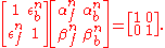
Levinson-Durbin recursion defines the nth "forward vector", denoted , as the vector of length n which satisfies:

The nth "backward vector" is defined similarly; it is the vector of length n which satisfies:

An important simplification can occur when M is a symmetric matrix; then the two vectors are related by bni = fnn+1-i -- that is, they are row-reversals of each other. This can save some extra computation in that special case.
Obtaining the backward vectors
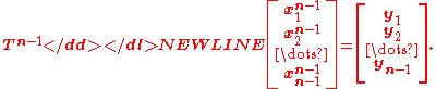
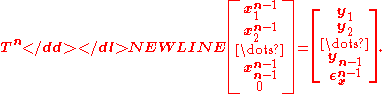
Even if the matrix is not symmetric, then the nth forward and backward vector may be found from the vectors of length n-1 as follows. First, the forward vector may be extended with a zero to obtain:
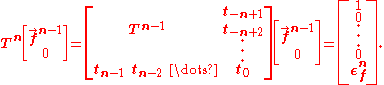
In going from Tn-1 to Tn, the extra column added to the matrix does not perturb the solution when a zero is used to extend the forward vector. However, the extra row added to the matrix has perturbed the solution; and it has created an unwanted error term εf which occurs in the last place. The above equation gives it the value of:
This error will be returned to shortly and eliminated from the new forward vector; but first, the backwards vector must be extended in a similar (albeit reversed) fashion. For the backwards vector,
Like before, the extra column added to the matrix does not perturb this new backwards vector; but the extra row does. Here we have another unwanted error εb with value:

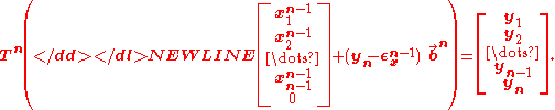
These two error terms can be used to eliminate each other. Using the linearity of matrices,
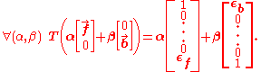
If α and β are chosen so that the right hand side yields ê1 or ên, then the quantity in the parentheses will fulfill the definition of the nth forward or backward vector, respectively. With those alpha and beta chosen, the vector sum in the parentheses is simple and yields the desired result.
To find these coefficients, ,
,  are such that :
and respectively ,
,  are such that :
By multiplying both previous equations by one gets the following equation:
-
Now, all the zeroes in the middle of the two vectors above being disregarded and collapsed, only the following equation is left:
With these solved for (by using the Cramer 2x2 matrix inverse formula), the new forward and backward vectors are:
-

-

Performing these vector summations, then, gives the nth forward and backward vectors from the prior ones. All that remains is to find the first of these vectors, and then some quick sums and multiplications give the remaining ones. The first forward and backward vectors are simply:
Using the backward vectors
The above steps give the N backward vectors for M. From there, a more arbitrary equation is:
The solution can be built in the same recursive way that the backwards vectors were built. Accordingly, must be generalized to a sequence
  , from which
  .
.
The solution is then built recursively by noticing that if:
-
Then, extending with a zero again, and defining an error constant where necessary:
-
We can then use the nth backward vector to eliminate the error term and replace it with the desired formula as follows:
-
Extending this method until n = N yields the solution .
.
In practice, these steps are often done concurrently with the rest of the procedure, but they form a coherent unit and deserve to be treated as their own step.
Block Levinson algorithm
If M is not strictly Toeplitz, but blockBlock matrixIn the mathematical discipline of matrix theory, a block matrix or a partitioned matrix is a matrix broken into sections called blocks. Looking at it another way, the matrix is written in terms of smaller matrices. We group the rows and columns into adjacent 'bunches'. A partition is the rectangle...
Toeplitz, the Levinson recursion can be derived in much the same way by regarding the block Toeplitz matrix as a Toeplitz matrix with matrix elements (Musicus 1988). Block Toeplitz matrices arise naturally in signal processing algorithms when dealing with multiple signal streams (e.g., in MIMO systems) or cyclo-stationary signals.
-
-
-
-
-
-