Hasegawa-Mima equation - AbsoluteAstronomy.com

In plasma physics, the Hasegawa–Mima equation, named after Akira Hasegawa and Kunioki Mima, is an equation that describes a certain regime of plasma

Plasma (physics)

In physics and chemistry, plasma is a state of matter similar to gas in which a certain portion of the particles are ionized. Heating a gas may ionize its molecules or atoms , thus turning it into a plasma, which contains charged particles: positive ions and negative electrons or ions...

, where the time scales are very fast, and the distance scale in the direction of the magnetic field is long. In particular the equation is useful for describing turbulence in some tokamak

Tokamak

A tokamak is a device using a magnetic field to confine a plasma in the shape of a torus . Achieving a stable plasma equilibrium requires magnetic field lines that move around the torus in a helical shape...

s. The equation was introduced in Hasegawa and Mima's paper submitted in 1977 to Physics of Fluids, where they compared it to the results of the ATC tokamak.

Assumptions

The magnetic field is large enough that:

for all quantities of interest. When the particles in the plasma are moving through a magnetic field, they spin in a circle around the magnetic field. The frequency of oscillation,

known as the cyclotron frequency or gyrofrequency, is directly proportional to the magnetic field.

The particle density follows the quasineutrality condition:

where Z is the number of protons in the ions. If we are talking about hydrogen Z = 1, and n is the same for both species. This condition is true as long as the electrons can shield out electric fields. A cloud of electrons will surround any charge with an approximate radius known as the Debye length

Debye length

In plasma physics, the Debye length , named after the Dutch physicist and physical chemist Peter Debye, is the scale over which mobile charge carriers screen out electric fields in plasmas and other conductors. In other words, the Debye length is the distance over which significant charge...

. For that reason this approximation means the size scale is much larger than the Debye length. The ion particle density can be expressed by a first order term that is the density defined by the quasineutrality condition equation, and a second order term which is how much it differs from the equation.

The first order ion particle density is a function of position, but not time. This means that perturbations of the particle density change at a timescale much slower than the scale of interest. The second order particle density which causes a charge density and thus an electric potential can change with time.

The magnetic field, B must be uniform in space, and not be a function of time. The magnetic field also moves at a timescale much slower than the scale of interest. This allows the time derivative in the momentum balance equation to be neglected.

The ion temperature must be much smaller than the electron temperature. This means that the ion pressure can be neglected in the ion momentum balance equation.

The electrons follow a Boltzmann distribution
Boltzmann distribution
In chemistry, physics, and mathematics, the Boltzmann distribution is a certain distribution function or probability measure for the distribution of the states of a system. It underpins the concept of the canonical ensemble, providing its underlying distribution...

where:

Since the electrons are free to move along the direction of the magnetic field, they screen away electric potentials. This screening causes a Boltzmann distribution of electrons to form around the electric potentials.

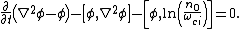
The equation

The Hasegawa–Mima equation is a second order nonlinear partial differential equation that describes the electric potential. The form of the equation is:

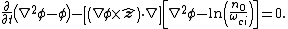
Although the quasi neutrality condition holds, the small differences in density between the electrons and the ions cause an electric potential.
The Hasegawa–Mima equation is derived from the continuity equation:

The fluid velocity can be approximated by the E cross B drift:

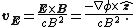
Previous models derived their equations from this approximation. The divergence of the E cross B drift is zero, which keeps the fluid incompressible. However, the compressibility of the fluid is very important in describing the evolution of the system. Hasegawa and Mima argued that the assumption was invalid. The Hasegawa–Mima equation introduces a second order term for the fluid velocity known as the polarization drift in order to find the divergence of the fluid velocity. Due to the assumption of large magnetic field, the polarization drift is much smaller than the E cross B drift. Nevertheless, it introduces important physics.

For a two-dimensional incompressible fluid which is not a plasma, the Navier–Stokes equations say:

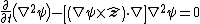
after taking the curl of the momentum balance equation. This equation is almost identical to the Hasegawa–Mima equation except the second and fourth terms are gone, and the electric potential is replaced with the fluid velocity vector potential where:

The first and third terms to the Hasegawa–Mima equation, which are the same as the Navier Stokes equation, are the terms introduced by adding the polarization drift. In the limit where the wavelength of a perturbation of the electric potential is much smaller than the gyroradius based on the sound speed, the Hasegawa–Mima equations become the same as the two-dimensional incompressible fluid.

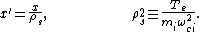
Normalization

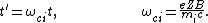
One way to understand an equation more fully is to understand what it is normalized to, which gives you an idea of the scales of interest. The time, position, and electric potential are normalized to t',x', and

The time scale for the Hasegawa–Mima equation is the inverse ion gyrofrequency:

From the large magnetic field assumption the normalized time is very small. However, it is still large enough to get information out of it.

The distance scale is the gyroradius based on the sound speed:

If you transform to k-space, it is clear that when k, the wavenumber, is much larger than one, the terms that make the Hasegawa–Mima equation differ from the equation derived from Navier-Stokes equation in a two dimensional incompressible flow become much smaller than the rest.

From the distance and time scales we can determine the scale for velocities. This turns out to be the sound speed. The Hasegawa–Mima equation, shows us the dynamics of fast moving sounds as opposed to the slower dynamics such as flows that are captured in the MHD equations

Magnetohydrodynamics

Magnetohydrodynamics is an academic discipline which studies the dynamics of electrically conducting fluids. Examples of such fluids include plasmas, liquid metals, and salt water or electrolytes...

. The motion is even faster than the sound speed given that the time scales are much smaller than the time normalization.

The potential is normalized to:

Since the electrons fit a Maxwellian

Maxwellian

* Maxwell's equations * Maxwell–Boltzmann distribution* Maxwell's electromagnetic wave equation...

and the quasineutrality condition holds, this normalized potential is small, but similar order to the normalized time derivative.

The entire equation without normalization is:

Although the time derivative divided by the cyclotron frequency is much smaller than unity, and the normalized electric potential is much smaller than unity, as long as the gradient is on the order of one, both terms are comparable to the nonlinear term. The unperturbed density gradient can also be just as small as the normalized electric potential and be comparable to the other terms.

Other forms of the equation

Often the Hasegawa–Mima equation is expressed in a different form using Poisson brackets. These Poisson brackets are defined as:

Using these Poisson brackets, the equation can be reexpressed as:

Often the particle density is assumed to vary uniformly just in one direction, and the equation is written in a sightly different form. The Poisson bracket including the density is replaced with the definition of the Poisson bracket, and a constant replaces the derivative of the density dependent term.

Conserved quantities

There are two quantities that are conserved in a two-dimensional incompressible fluid.
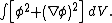
The kinetic energy

Kinetic energy

The kinetic energy of an object is the energy which it possesses due to its motion.It is defined as the work needed to accelerate a body of a given mass from rest to its stated velocity. Having gained this energy during its acceleration, the body maintains this kinetic energy unless its speed changes...

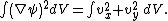
And the enstrophy:

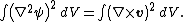
For the Hasegawa–Mima equation, there are also two conserved quantities, that are related to the above quantities. The generalized energy:

And the generalized enstrophy:

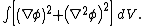
In the limit where the Hasegawa–Mima equation is the same as an incompressible fluid, the generalized energy, and enstrophy become the same as the kinetic energy and enstrophy.

Assumptions

The equation

Normalization

Other forms of the equation

Conserved quantities

See also