
Finite difference method
Encyclopedia
In mathematics
, finite-difference methods are numerical methods for approximating the solutions to differential equations using finite difference
equations to approximate derivatives.
,

where n! denotes the factorial
of n, and Rn(x) is a remainder term, denoting the difference between the Taylor polynomial of degree n and the original function. Again using the first derivative of the function f as an example, by Taylor's theorem,

Setting, x0=a and (x-a)=h we have,

Dividing across by h gives:

Solving for f'(a):

so that for sufficiently small,

, the loss of precision due to computer rounding of decimal quantities, and truncation error
or discretization error
, the difference between the exact solution of the finite difference equation and the exact quantity assuming perfect arithmetic (that is, assuming no round-off).
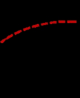
To use a finite difference method to attempt to solve (or, more generally, approximate the solution to) a problem, one must first discretize the problem's domain. This is usually done by dividing the domain into a uniform grid (see image to the right). Note that this means that finite-difference methods produce sets of discrete numerical approximations to the derivative, often in a "time-stepping" manner.
An expression of general interest is the local truncation error of a method. Typically expressed using Big-O notation, local truncation error refers to the error from a single application of a method. That is, it is the quantity if
if  refers to the exact value and
  to the numerical approximation. The remainder term of a Taylor polynomial is convenient for analyzing the local truncation error. Using the Lagrange form of the remainder from the Taylor polynomial for
  , which is
 , where
  ,
,
the dominant term of the local truncation error can be discovered. For example, again using the forward-difference formula for the first derivative, knowing that ,
,

and with some algebraic manipulation, this leads to

and further noting that the quantity on the left is the approximation from the finite difference method and that the quantity on the right is the exact quantity of interest plus a remainder, clearly that remainder is the local truncation error. A final expression of this example and its order is:

This means that, in this case, the local truncation error is proportional to the step size.

The Euler method for solving this equation uses the finite difference quotient
to approximate the differential equation by first substituting in for u'(x) and applying a little algebra to get
The last equation is a finite-difference equation, and solving this equation gives an approximate solution to the differential equation.
in one dimension, with homogeneous Dirichlet boundary condition
s

 (boundary condition)
 (initial condition)
One way to numerically solve this equation is to approximate all the derivatives by finite differences. We partition the domain in space using a mesh and in time using a mesh
  . We assume a uniform partition both in space and in time, so the difference between two consecutive space points will be h and between two consecutive time points will be k. The points

will represent the numerical approximation of
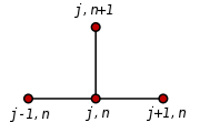 Using a forward difference at time
  and a second-order central difference for the space derivative at position
  ("FTCS") we get the recurrence equation:

This is an explicit method for solving the one-dimensional heat equation
.
We can obtain from the other values this way:

where
So, with this recurrence relation, and knowing the values at time n, one can obtain the corresponding values at time n+1. and
and  must be replaced by the boundary conditions, in this example they are both 0.
This explicit method is known to be numerically stable and convergent
whenever . The numerical errors are proportional to the time step and the square of the space step:
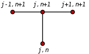 If we use the backward difference at time
  and a second-order central difference for the space derivative at position
  ("BTCS") we get the recurrence equation:

This is an implicit method for solving the one-dimensional heat equation
.
We can obtain from solving a system of linear equations:

The scheme is always numerically stable and convergent but usually more numerically intensive than the explicit method as it requires solving a system of numerical equations on each time step. The errors are linear over the time step and quadratic over the space step.
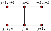
 and a second-order central difference for the space derivative at position
  ("CTCS") we get the recurrence equation:

This formula is known as the Crank–Nicolson method.
 We can obtain
  from solving a system of linear equations:

The scheme is always numerically stable and convergent but usually more numerically intensive as it requires solving a system of numerical equations on each time step. The errors are quadratic over the time step and formally are of the fourth degree regarding the space step:
However, near the boundaries, the error is often O(h2) instead of O(h4).
Usually the Crank–Nicolson scheme is the most accurate scheme for small time steps. The explicit scheme is the least accurate and can be unstable, but is also the easiest to implement and the least numerically intensive. The implicit scheme works the best for large time steps.
Mathematics
Mathematics is the study of quantity, space, structure, and change. Mathematicians seek out patterns and formulate new conjectures. Mathematicians resolve the truth or falsity of conjectures by mathematical proofs, which are arguments sufficient to convince other mathematicians of their validity...
, finite-difference methods are numerical methods for approximating the solutions to differential equations using finite difference
Finite difference
A finite difference is a mathematical expression of the form f − f. If a finite difference is divided by b − a, one gets a difference quotient...
equations to approximate derivatives.
Derivation from Taylor's polynomial
Assuming the function whose derivatives are to be approximated is properly-behaved, by Taylor's theoremTaylor's theorem
In calculus, Taylor's theorem gives an approximation of a k times differentiable function around a given point by a k-th order Taylor-polynomial. For analytic functions the Taylor polynomials at a given point are finite order truncations of its Taylor's series, which completely determines the...
,
where n! denotes the factorial
Factorial
In mathematics, the factorial of a non-negative integer n, denoted by n!, is the product of all positive integers less than or equal to n...
of n, and Rn(x) is a remainder term, denoting the difference between the Taylor polynomial of degree n and the original function. Again using the first derivative of the function f as an example, by Taylor's theorem,
Setting, x0=a and (x-a)=h we have,
Dividing across by h gives:
Solving for f'(a):
so that for
sufficiently small,Accuracy and order
The error in a method's solution is defined as the difference between its approximation and the exact analytical solution. The two sources of error in finite difference methods are round-off errorRound-off error
A round-off error, also called rounding error, is the difference between the calculated approximation of a number and its exact mathematical value. Numerical analysis specifically tries to estimate this error when using approximation equations and/or algorithms, especially when using finitely many...
, the loss of precision due to computer rounding of decimal quantities, and truncation error
Truncation error
Truncation error or local truncation error is error made by numerical algorithms that arises from taking finite number of steps in computation...
or discretization error
Discretization error
In numerical analysis, computational physics, and simulation, discretization error is error resulting from the fact that a function of a continuous variable is represented in the computer by a finite number of evaluations, for example, on a lattice...
, the difference between the exact solution of the finite difference equation and the exact quantity assuming perfect arithmetic (that is, assuming no round-off).
To use a finite difference method to attempt to solve (or, more generally, approximate the solution to) a problem, one must first discretize the problem's domain. This is usually done by dividing the domain into a uniform grid (see image to the right). Note that this means that finite-difference methods produce sets of discrete numerical approximations to the derivative, often in a "time-stepping" manner.
An expression of general interest is the local truncation error of a method. Typically expressed using Big-O notation, local truncation error refers to the error from a single application of a method. That is, it is the quantity
if refers to the exact value and to the numerical approximation. The remainder term of a Taylor polynomial is convenient for analyzing the local truncation error. Using the Lagrange form of the remainder from the Taylor polynomial for , which is, where ,the dominant term of the local truncation error can be discovered. For example, again using the forward-difference formula for the first derivative, knowing that
,and with some algebraic manipulation, this leads to
and further noting that the quantity on the left is the approximation from the finite difference method and that the quantity on the right is the exact quantity of interest plus a remainder, clearly that remainder is the local truncation error. A final expression of this example and its order is:
This means that, in this case, the local truncation error is proportional to the step size.
Example: ordinary differential equation
For example, consider the ordinary differential equationThe Euler method for solving this equation uses the finite difference quotient
to approximate the differential equation by first substituting in for u'(x) and applying a little algebra to get
The last equation is a finite-difference equation, and solving this equation gives an approximate solution to the differential equation.
Example: The heat equation
Consider the normalized heat equationHeat equation
The heat equation is an important partial differential equation which describes the distribution of heat in a given region over time...
in one dimension, with homogeneous Dirichlet boundary condition
Dirichlet boundary condition
In mathematics, the Dirichlet boundary condition is a type of boundary condition, named after Johann Peter Gustav Lejeune Dirichlet who studied under Cauchy and succeeded Gauss at University of Göttingen. When imposed on an ordinary or a partial differential equation, it specifies the values a...
s
(boundary condition) (initial condition)One way to numerically solve this equation is to approximate all the derivatives by finite differences. We partition the domain in space using a mesh
and in time using a mesh . We assume a uniform partition both in space and in time, so the difference between two consecutive space points will be h and between two consecutive time points will be k. The pointswill represent the numerical approximation of
Explicit method
and a second-order central difference for the space derivative at position ("FTCS") we get the recurrence equation:This is an explicit method for solving the one-dimensional heat equation
Heat equation
The heat equation is an important partial differential equation which describes the distribution of heat in a given region over time...
.
We can obtain
from the other values this way:where
So, with this recurrence relation, and knowing the values at time n, one can obtain the corresponding values at time n+1.
and must be replaced by the boundary conditions, in this example they are both 0.This explicit method is known to be numerically stable and convergent
Limit of a sequence
The limit of a sequence is, intuitively, the unique number or point L such that the terms of the sequence become arbitrarily close to L for "large" values of n...
whenever
. The numerical errors are proportional to the time step and the square of the space step:Implicit method
and a second-order central difference for the space derivative at position ("BTCS") we get the recurrence equation:This is an implicit method for solving the one-dimensional heat equation
Heat equation
The heat equation is an important partial differential equation which describes the distribution of heat in a given region over time...
.
We can obtain
from solving a system of linear equations:The scheme is always numerically stable and convergent but usually more numerically intensive than the explicit method as it requires solving a system of numerical equations on each time step. The errors are linear over the time step and quadratic over the space step.
Crank–Nicolson method
Finally if we use the central difference at time and a second-order central difference for the space derivative at position ("CTCS") we get the recurrence equation:This formula is known as the Crank–Nicolson method.
from solving a system of linear equations:The scheme is always numerically stable and convergent but usually more numerically intensive as it requires solving a system of numerical equations on each time step. The errors are quadratic over the time step and formally are of the fourth degree regarding the space step:
However, near the boundaries, the error is often O(h2) instead of O(h4).
Usually the Crank–Nicolson scheme is the most accurate scheme for small time steps. The explicit scheme is the least accurate and can be unstable, but is also the easiest to implement and the least numerically intensive. The implicit scheme works the best for large time steps.
See also
- Difference operator
- Stencil (numerical analysis)Stencil (numerical analysis)In mathematics, especially the areas of numerical analysis concentrating on the numerical solution of partial differential equations, a stencil is a geometric arrangement of a nodal group that relate to the point of interest by using a numerical approximation routine. Stencils are the basis for...
- Finite difference coefficients
- Five-point stencilFive-point stencilIn numerical analysis, given a square grid in one or two dimensions, the five-point stencil of a point in the grid is made up of the point itself together with its four "neighbors"...
- Lax–Richtmyer theorem
- Finite difference methods for option pricingFinite difference methods for option pricingFinite difference methods for option pricing are numerical methods used in mathematical finance for the valuation of options. Finite difference methods were first applied to option pricing by Eduardo Schwartz in 1977....
External links
- List of Internet Resources for the Finite Difference Method for PDEs
- Finite Difference Method of Solving ODEs (Boundary Value Problems) Notes, PPT, Maple, Mathcad, Matlab, Mathematica
- Lecture Notes Shih-Hung Chen, National Central UniversityNational Central UniversityNational Central University is a national comprehensive university in Taiwan .National Central University was founded in 1915 and originated in 258 CE at Nanjing, China. After NCU in Nanjing was renamed Nanjing University in 1949, NCU was re-established in Taiwan in 1962...
- Lecture Notes Randall J. LeVeque University of WashingtonUniversity of WashingtonUniversity of Washington is a public research university, founded in 1861 in Seattle, Washington, United States. The UW is the largest university in the Northwest and the oldest public university on the West Coast. The university has three campuses, with its largest campus in the University...
- Finite Difference Method
- Finite Difference Method for Boundary Value Problems
- Finite Difference Methodology in Materials Science