

Derivation of the conjugate gradient method
Encyclopedia
In numerical linear algebra
, the conjugate gradient method
is an iterative method
for numerically solving the linear system

where is symmetric positive-definite
. The conjugate gradient method can be derived from several different perspectives, including specialization of the conjugate direction method for optimization
, and variation of the Arnoldi
/Lanczos iteration for eigenvalue problems.
The intent of this article is to document the important steps in these derivations.


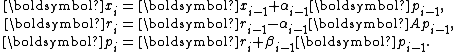
one starts with an initial guess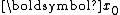 and the corresponding residual
  , and computes the iterate and residual by the formulae
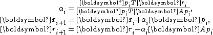
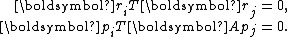
where are a series of mutually conjugate directions, i.e.,

for any .
.
The conjugate direction method is imprecise in the sense that no formulae are given for selection of the directions . Specific choices lead to various methods including the conjugate gradient method and Gaussian elimination
.
 and gradually builds an orthonormal basis
  of the Krylov subspace

by defining where
where

In other words, for ,
,  is found by Gram-Schmidt orthogonalizing
  against
  followed by normalization.
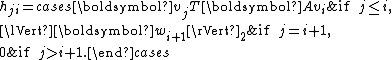
Put in matrix form, the iteration is captured by the equation

where
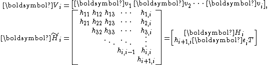
with
When applying the Arnoldi iteration to solving linear systems, one starts with , the residual corresponding to an initial guess
  . After each step of iteration, one computes
  and the new iterate
  .
.
 is symmetric positive-definite. With symmetry of
  , the upper Hessenberg matrix
  becomes symmetric and thus tridiagonal. It then can be more clearly denoted by
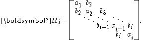
This enables a short three-term recurrence for in the iteration, and the Arnoldi iteration is reduced to the Lanczos iteration.
Since is symmetric positive-definite, so is
 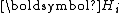 . Hence,
  can be LU factorized without partial pivoting into
with convenient recurrences for and
and  :
:
Rewrite as
as

with

It is now important to observe that
In fact, there are short recurrences for and
and  as well:

With this formulation, we arrive at a simple recurrence for :
:

The relations above straightforwardly lead to the direct Lanczos method, which turns out to be slightly more complex.
 to scale and compensate for the scaling in the constant factor, we potentially can have simpler recurrences of the form:
As premises for the simplification, we now derive the orthogonality of and conjugacy of
  , i.e., for
  ,
,
The residuals are mutually orthogonal because is essentially a multiple of
  since for
  ,
,  , for
, for  ,
,

To see the conjugacy of , it suffices to show that
  is diagonal:
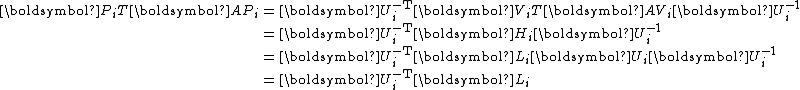
is symmetric and lower triangular simultaneously and thus must be diagonal.
Now we can derive the constant factors and
and  with respect to the scaled
  by solely imposing the orthogonality of
  and conjugacy of
  .
.
Due to the orthogonality of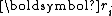 , it is necessary that
  . As a result,
Similarly, due to the conjugacy of , it is necessary that
  . As a result,
This completes the derivation.
Numerical linear algebra
Numerical linear algebra is the study of algorithms for performing linear algebra computations, most notably matrix operations, on computers. It is often a fundamental part of engineering and computational science problems, such as image and signal processing, Telecommunication, computational...
, the conjugate gradient method
Conjugate gradient method
In mathematics, the conjugate gradient method is an algorithm for the numerical solution of particular systems of linear equations, namely those whose matrix is symmetric and positive-definite. The conjugate gradient method is an iterative method, so it can be applied to sparse systems that are too...
is an iterative method
Iterative method
In computational mathematics, an iterative method is a mathematical procedure that generates a sequence of improving approximate solutions for a class of problems. A specific implementation of an iterative method, including the termination criteria, is an algorithm of the iterative method...
for numerically solving the linear system
where
is symmetric positive-definitePositive-definite matrix
In linear algebra, a positive-definite matrix is a matrix that in many ways is analogous to a positive real number. The notion is closely related to a positive-definite symmetric bilinear form ....
. The conjugate gradient method can be derived from several different perspectives, including specialization of the conjugate direction method for optimization
Optimization (mathematics)
In mathematics, computational science, or management science, mathematical optimization refers to the selection of a best element from some set of available alternatives....
, and variation of the Arnoldi
Arnoldi iteration
In numerical linear algebra, the Arnoldi iteration is an eigenvalue algorithm and an important example of iterative methods. Arnoldi finds the eigenvalues of general matrices; an analogous method for Hermitian matrices is the Lanczos iteration. The Arnoldi iteration was invented by W. E...
/Lanczos iteration for eigenvalue problems.
The intent of this article is to document the important steps in these derivations.
Derivation from the conjugate direction method
The conjugate gradient method can be seen as a special case of the conjugate direction method applied to minimization of the quadratic functionThe conjugate direction method
In the conjugate direction method for minimizingone starts with an initial guess
and the corresponding residual , and computes the iterate and residual by the formulaewhere
are a series of mutually conjugate directions, i.e.,for any
.The conjugate direction method is imprecise in the sense that no formulae are given for selection of the directions
. Specific choices lead to various methods including the conjugate gradient method and Gaussian eliminationGaussian elimination
In linear algebra, Gaussian elimination is an algorithm for solving systems of linear equations. It can also be used to find the rank of a matrix, to calculate the determinant of a matrix, and to calculate the inverse of an invertible square matrix...
.
Derivation from the Arnoldi/Lanczos iteration
The conjugate gradient method can also be seen as a variant of the Arnoldi/Lanczos iteration applied to solving linear systems.The general Arnoldi method
In the Arnoldi iteration, one starts with a vector and gradually builds an orthonormal basis of the Krylov subspaceKrylov subspace
In linear algebra, the order-r Krylov subspace generated by an n-by-n matrix A and a vector b of dimension n is the linear subspace spanned by the images of b under the first r powers of A , that is,...
by defining
whereIn other words, for
, is found by Gram-Schmidt orthogonalizing against followed by normalization.Put in matrix form, the iteration is captured by the equation
where
with
When applying the Arnoldi iteration to solving linear systems, one starts with
, the residual corresponding to an initial guess . After each step of iteration, one computes and the new iterate .The direct Lanzcos method
For the rest of discussion, we assume that is symmetric positive-definite. With symmetry of , the upper Hessenberg matrix becomes symmetric and thus tridiagonal. It then can be more clearly denoted byThis enables a short three-term recurrence for
in the iteration, and the Arnoldi iteration is reduced to the Lanczos iteration.Since
is symmetric positive-definite, so is . Hence, can be LU factorized without partial pivoting intowith convenient recurrences for
and :Rewrite
aswith
It is now important to observe that
In fact, there are short recurrences for
and as well:With this formulation, we arrive at a simple recurrence for
:The relations above straightforwardly lead to the direct Lanczos method, which turns out to be slightly more complex.
The conjugate gradient method from imposing orthogonality and conjugacy
If we allow to scale and compensate for the scaling in the constant factor, we potentially can have simpler recurrences of the form:As premises for the simplification, we now derive the orthogonality of
and conjugacy of , i.e., for ,The residuals are mutually orthogonal because
is essentially a multiple of since for , , for ,To see the conjugacy of
, it suffices to show that is diagonal:is symmetric and lower triangular simultaneously and thus must be diagonal.
Now we can derive the constant factors
and with respect to the scaled by solely imposing the orthogonality of and conjugacy of .Due to the orthogonality of
, it is necessary that . As a result,Similarly, due to the conjugacy of
, it is necessary that . As a result,This completes the derivation.