

Bruun's FFT algorithm
Encyclopedia
Bruun's algorithm is a fast Fourier transform
(FFT) algorithm based on an unusual recursive polynomial
-factorization approach, proposed for powers of two by G. Bruun in 1978 and generalized to arbitrary even composite sizes by H. Murakami in 1996. Because its operations involve only real coefficients until the last computation stage, it was initially proposed as a way to efficiently compute the discrete Fourier transform
(DFT) of real data. Bruun's algorithm has not seen widespread use, however, as approaches based on the ordinary Cooley–Tukey FFT algorithm have been successfully adapted to real data with at least as much efficiency. Furthermore, there is evidence that Bruun's algorithm may be intrinsically less accurate than Cooley–Tukey in the face of finite numerical precision (Storn, 1993).
Nevertheless, Bruun's algorithm illustrates an alternative algorithmic framework that can express both itself and the Cooley–Tukey algorithm, and thus provides an interesting perspective on FFTs that permits mixtures of the two algorithms and other generalizations.
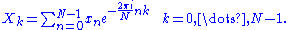
For convenience, let us denote the N roots of unity
by ωNn (n = 0, ..., N − 1):

and define the polynomial x(z) whose coefficients are xn:

The DFT can then be understood as a reduction of this polynomial; that is, Xk is given by:

where mod denotes the polynomial remainder
operation. The key to fast algorithms like Bruun's or Cooley–Tukey comes from the fact that one can perform this set of N remainder operations in recursive stages.
 modulo N degree-1 polynomials as described above. Evaluating these remainders one by one is equivalent to the evaluating the usual DFT formula directly, and requires O(N2) operations. However, one can combine these remainders recursively to reduce the cost, using the following trick: if we want to evaluate
  modulo two polynomials
  and
and  , we can first take the remainder modulo their product
 , which reduces the degree
of the polynomial and makes subsequent modulo operations less computationally expensive.
The product of all of the monomials for k=0..N-1 is simply
  (whose roots are clearly the N roots of unity). One then wishes to find a recursive factorization of
  into polynomials of few terms and smaller and smaller degree. To compute the DFT, one takes
  modulo each level of this factorization in turn, recursively, until one arrives at the monomials and the final result. If each level of the factorization splits every polynomial into an O(1) (constant-bounded) number of smaller polynomials, each with an O(1) number of nonzero coefficients, then the modulo operations for that level take O(N) time; since there will be a logarithmic number of levels, the overall complexity is O (N log N).
More explicitly, suppose for example that , and that
 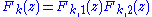 , and so on. The corresponding FFT algorithm would consist of first computing xk(z) = x(z) mod
Fk(z), then computing xk,j(z) = xk(z) mod
Fk,j(z), and so on, recursively creating more and more remainder polynomials of smaller and smaller degree until one arrives at the final degree-0 results.
Moreover, as long as the polynomial factors at each stage are relatively prime (which for polynomials means that they have no common roots), one can construct a dual algorithm by reversing the process with the Chinese Remainder Theorem
.
 into
into  and
and  . These modulo operations reduce the degree of
  by 2, which corresponds to dividing the problem size by 2. Instead of recursively factorizing
  directly, though, Cooley–Tukey instead first computes x2(z ωN), shifting all the roots (by a twiddle factor) so that it can apply the recursive factorization of
  to both subproblems. That is, Cooley–Tukey ensures that all subproblems are also DFTs, whereas this is not generally true for an arbitrary recursive factorization (such as Bruun's, below).
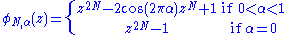
factorizes zN-1 recursively via the rules:


where a is a real constant with |a| ≤ 2. At the end of the recursion, for M=1, you are left with degree-2 polynomials that can then be evaluated modulo two roots (z - ωNk) for each polynomial. Thus, at each recursive stage, all of the polynomials are factorized into two parts of half the degree, each of which has at most three nonzero terms, leading to an O (N log N) algorithm for the FFT.
Moreover, since all of these polynomials have purely real coefficients (until the very last stage), they automatically exploit the special case where the inputs xn are purely real to save roughly a factor of two in computation and storage. One can also take straightforward advantage of the case of real-symmetric data for computing the discrete cosine transform
(Chen and Sorensen, 1992).
[0,1) by:
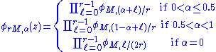
Note that all of the polynomials that appear in the Bruun factorization above can be written in this form. These polynomials can be recursively factorized for a factor (radix) r via:
Fast Fourier transform
A fast Fourier transform is an efficient algorithm to compute the discrete Fourier transform and its inverse. "The FFT has been called the most important numerical algorithm of our lifetime ." There are many distinct FFT algorithms involving a wide range of mathematics, from simple...
(FFT) algorithm based on an unusual recursive polynomial
Polynomial
In mathematics, a polynomial is an expression of finite length constructed from variables and constants, using only the operations of addition, subtraction, multiplication, and non-negative integer exponents...
-factorization approach, proposed for powers of two by G. Bruun in 1978 and generalized to arbitrary even composite sizes by H. Murakami in 1996. Because its operations involve only real coefficients until the last computation stage, it was initially proposed as a way to efficiently compute the discrete Fourier transform
Discrete Fourier transform
In mathematics, the discrete Fourier transform is a specific kind of discrete transform, used in Fourier analysis. It transforms one function into another, which is called the frequency domain representation, or simply the DFT, of the original function...
(DFT) of real data. Bruun's algorithm has not seen widespread use, however, as approaches based on the ordinary Cooley–Tukey FFT algorithm have been successfully adapted to real data with at least as much efficiency. Furthermore, there is evidence that Bruun's algorithm may be intrinsically less accurate than Cooley–Tukey in the face of finite numerical precision (Storn, 1993).
Nevertheless, Bruun's algorithm illustrates an alternative algorithmic framework that can express both itself and the Cooley–Tukey algorithm, and thus provides an interesting perspective on FFTs that permits mixtures of the two algorithms and other generalizations.
A polynomial approach to the DFT
Recall that the DFT is defined by the formula:For convenience, let us denote the N roots of unity
Root of unity
In mathematics, a root of unity, or de Moivre number, is any complex number that equals 1 when raised to some integer power n. Roots of unity are used in many branches of mathematics, and are especially important in number theory, the theory of group characters, field theory, and the discrete...
by ωNn (n = 0, ..., N − 1):
and define the polynomial x(z) whose coefficients are xn:
The DFT can then be understood as a reduction of this polynomial; that is, Xk is given by:
where mod denotes the polynomial remainder
Polynomial remainder theorem
In algebra, the polynomial remainder theorem or little Bézout's theorem is an application of polynomial long division. It states that the remainder of a polynomial f\, divided by a linear divisor x-a\, is equal to f \,.- Example :...
operation. The key to fast algorithms like Bruun's or Cooley–Tukey comes from the fact that one can perform this set of N remainder operations in recursive stages.
Recursive factorizations and FFTs
In order to compute the DFT, we need to evaluate the remainder of modulo N degree-1 polynomials as described above. Evaluating these remainders one by one is equivalent to the evaluating the usual DFT formula directly, and requires O(N2) operations. However, one can combine these remainders recursively to reduce the cost, using the following trick: if we want to evaluate modulo two polynomials and , we can first take the remainder modulo their product , which reduces the degreeDegree (mathematics)
In mathematics, there are several meanings of degree depending on the subject.- Unit of angle :A degree , usually denoted by ° , is a measurement of a plane angle, representing 1⁄360 of a turn...
of the polynomial
and makes subsequent modulo operations less computationally expensive.The product of all of the monomials
for k=0..N-1 is simply (whose roots are clearly the N roots of unity). One then wishes to find a recursive factorization of into polynomials of few terms and smaller and smaller degree. To compute the DFT, one takes modulo each level of this factorization in turn, recursively, until one arrives at the monomials and the final result. If each level of the factorization splits every polynomial into an O(1) (constant-bounded) number of smaller polynomials, each with an O(1) number of nonzero coefficients, then the modulo operations for that level take O(N) time; since there will be a logarithmic number of levels, the overall complexity is O (N log N).More explicitly, suppose for example that
, and that , and so on. The corresponding FFT algorithm would consist of first computing xk(z) = x(z) modFk(z), then computing xk,j(z) = xk(z) mod
Fk,j(z), and so on, recursively creating more and more remainder polynomials of smaller and smaller degree until one arrives at the final degree-0 results.
Moreover, as long as the polynomial factors at each stage are relatively prime (which for polynomials means that they have no common roots), one can construct a dual algorithm by reversing the process with the Chinese Remainder Theorem
Chinese remainder theorem
The Chinese remainder theorem is a result about congruences in number theory and its generalizations in abstract algebra.In its most basic form it concerned with determining n, given the remainders generated by division of n by several numbers...
.
Cooley–Tukey as polynomial factorization
The standard decimation-in-frequency (DIF) radix-r Cooley–Tukey algorithm corresponds closely to a recursive factorization. For example, radix-2 DIF Cooley–Tukey factors into and . These modulo operations reduce the degree of by 2, which corresponds to dividing the problem size by 2. Instead of recursively factorizing directly, though, Cooley–Tukey instead first computes x2(z ωN), shifting all the roots (by a twiddle factor) so that it can apply the recursive factorization of to both subproblems. That is, Cooley–Tukey ensures that all subproblems are also DFTs, whereas this is not generally true for an arbitrary recursive factorization (such as Bruun's, below).The Bruun factorization
The basic Bruun algorithm for powers of twoPower of two
In mathematics, a power of two means a number of the form 2n where n is an integer, i.e. the result of exponentiation with as base the number two and as exponent the integer n....
factorizes zN-1 recursively via the rules:
where a is a real constant with |a| ≤ 2. At the end of the recursion, for M=1, you are left with degree-2 polynomials that can then be evaluated modulo two roots (z - ωNk) for each polynomial. Thus, at each recursive stage, all of the polynomials are factorized into two parts of half the degree, each of which has at most three nonzero terms, leading to an O (N log N) algorithm for the FFT.
Moreover, since all of these polynomials have purely real coefficients (until the very last stage), they automatically exploit the special case where the inputs xn are purely real to save roughly a factor of two in computation and storage. One can also take straightforward advantage of the case of real-symmetric data for computing the discrete cosine transform
Discrete cosine transform
A discrete cosine transform expresses a sequence of finitely many data points in terms of a sum of cosine functions oscillating at different frequencies. DCTs are important to numerous applications in science and engineering, from lossy compression of audio and images A discrete cosine transform...
(Chen and Sorensen, 1992).
Generalization to arbitrary radices
The Bruun factorization, and thus the Bruun FFT algorithm, was generalized to handle arbitrary even composite lengths, i.e. dividing the polynomial degree by an arbitrary radix (factor), as follows. First, we define a set of polynomials φN,α(z) for positive integers N and for α inNote that all of the polynomials that appear in the Bruun factorization above can be written in this form. These polynomials can be recursively factorized for a factor (radix) r via: