Pole splitting
Encyclopedia
Pole splitting is a phenomenon exploited in some forms of frequency compensation
used in an electronic amplifier
. When a capacitor
is introduced between the input and output sides of the amplifier with the intention of moving the pole lowest in frequency (usually an input pole) to lower frequencies, pole splitting causes the pole next in frequency (usually an output pole) to move to a higher frequency. This pole movement increases the stability of the amplifier and improves its step response
at the cost of decreased speed.
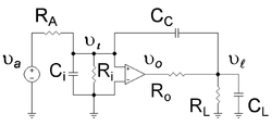
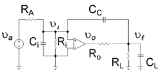
 This example shows that introduction of the capacitor referred to as CC in the amplifier of Figure 1 has two results: first it causes the lowest frequency pole of the amplifier to move still lower in frequency and second, it causes the higher pole to move higher in frequency. The amplifier of Figure 1 has a low frequency pole due to the added input resistance Ri and capacitance Ci, with the time constant Ci ( RA // Ri ). This pole is moved down in frequency by the Miller effect. The amplifier is given a high frequency output pole by addition of the load resistance RL and capacitance CL, with the time constant CL ( Ro // RL ). The upward movement of the high-frequency pole occurs because the Miller-amplified compensation capacitor CC alters the frequency dependence of the output voltage divider.
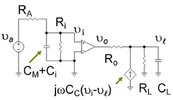
The first objective, to show the lowest pole moves down in frequency, is established using the same approach as the Miller's theorem
article. Following the procedure described in the article on Miller's theorem, the circuit of Figure 1 is transformed to that of Figure 2, which is electrically equivalent to Figure 1. Application of Kirchhoff's current law to the input side of Figure 2 determines the input voltage to the ideal op amp as a function of the applied signal voltage
  , namely,
Frequency compensation
In electrical engineering, frequency compensation is a technique used in amplifiers, and especially in amplifiers employing negative feedback. It usually has two primary goals: To avoid the unintentional creation of positive feedback, which will cause the amplifier to oscillate, and to control...
used in an electronic amplifier
Electronic amplifier
An electronic amplifier is a device for increasing the power of a signal.It does this by taking energy from a power supply and controlling the output to match the input signal shape but with a larger amplitude...
. When a capacitor
Capacitor
A capacitor is a passive two-terminal electrical component used to store energy in an electric field. The forms of practical capacitors vary widely, but all contain at least two electrical conductors separated by a dielectric ; for example, one common construction consists of metal foils separated...
is introduced between the input and output sides of the amplifier with the intention of moving the pole lowest in frequency (usually an input pole) to lower frequencies, pole splitting causes the pole next in frequency (usually an output pole) to move to a higher frequency. This pole movement increases the stability of the amplifier and improves its step response
Step response
The step response of a system in a given initial state consists of the time evolution of its outputs when its control inputs are Heaviside step functions. In electronic engineering and control theory, step response is the time behaviour of the outputs of a general system when its inputs change from...
at the cost of decreased speed.
Example of pole splitting
The first objective, to show the lowest pole moves down in frequency, is established using the same approach as the Miller's theorem
Miller effect
In electronics, the Miller effect accounts for the increase in the equivalent input capacitance of an inverting voltage amplifier due to amplification of the effect of capacitance between the input and output terminals...
article. Following the procedure described in the article on Miller's theorem, the circuit of Figure 1 is transformed to that of Figure 2, which is electrically equivalent to Figure 1. Application of Kirchhoff's current law to the input side of Figure 2 determines the input voltage
to the ideal op amp as a function of the applied signal voltage , namely,-

which exhibits a roll-offRoll-offRoll-off is a term commonly used to describe the steepness of a transmission function with frequency, particularly in electrical network analysis, and most especially in connection with filter circuits in the transition between a passband and a stopband...
with frequency beginning at f1 where
-

which introduces notation for the time constant of the lowest pole. This frequency is lower than the initial low frequency of the amplifier, which for CC = 0 F is
  .
.
Turning to the second objective, showing the higher pole moves still higher in frequency, it is necessary to look at the output side of the circuit, which contributes a second factor to the overall gain, and additional frequency dependence. The voltage is determined by the gain of the ideal op amp inside the amplifier as
Using this relation and applying Kirchhoff's current law to the output side of the circuit determines the load voltage as a function of the voltage
  at the input to the ideal op amp as:
This expression is combined with the gain factor found earlier for the input side of the circuit to obtain the overall gain as
-

This gain formula appears to show a simple two-pole response with two time constants. (It also exhibits a zero in the numerator but, assuming the amplifier gain Av is large, this zero is important only at frequencies too high to matter in this discussion , so the numerator can be approximated as unity.) However, although the amplifier does have a two-pole behavior, the two time-constants are more complicated than the above expression suggests because the Miller capacitance contains a buried frequency dependence that has no importance at low frequencies, but has considerable effect at high frequencies. That is, assuming the output R-C product, CL ( Ro // RL ), corresponds to a frequency well above the low frequency pole, the accurate form of the Miller capacitance must be used, rather than the Miller approximation. According to the article on Miller effect, the Miller capacitance is given by
-
(For a positive Miller capacitance, Av is negative.) Upon substitution of this result into the gain expression and collecting terms, the gain is rewritten as:
with Dω given by a quadratic in ω, namely:
Every quadratic has two factors, and this expression looks simpler if it is rewritten as
-

where and
and  are combinations of the capacitances and resistances in the formula for Dω. They correspond to the time constants of the two poles of the amplifier. One or the other time constant is the longest; suppose
  is the longest time constant, corresponding to the lowest pole, and suppose
  >>
>>  . (Good step response requires
  >>
>>  . See Selection of CC below.)
At low frequencies near the lowest pole of this amplifier, ordinarily the linear term in ω is more important than the quadratic term, so the low frequency behavior of Dω is:
-

where now CM is redefined using the Miller approximationMiller effectIn electronics, the Miller effect accounts for the increase in the equivalent input capacitance of an inverting voltage amplifier due to amplification of the effect of capacitance between the input and output terminals...
as
which is simply the previous Miller capacitance evaluated at low frequencies. On this basis is determined, provided
  >>
>>  . Because CM is large, the time constant
  is much larger than its original value of Ci ( RA // Ri ).
At high frequencies the quadratic term becomes important. Assuming the above result for is valid, the second time constant, the position of the high frequency pole, is found from the quadratic term in Dω as
Substituting in this expression the quadratic coefficient corresponding to the product along with the estimate for
  , an estimate for the position of the second pole is found:
-

and because CM is large, it seems is reduced in size from its original value CL ( Ro // RL ); that is, the higher pole has moved still higher in frequency because of CC.
In short, introduction of capacitor CC moved the low pole lower and the high pole higher, so the term pole splitting seems a good description.
Selection of CC
What value is a good choice for CC? For general purpose use, traditional design (often called dominant-pole or single-pole compensation) requires the amplifier gain to drop at 20 dB/decade from the corner frequency down to 0 dB gain, or even lower.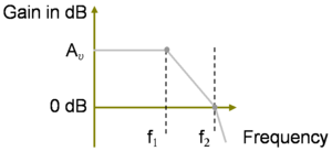
With this design the amplifier is stable and has near-optimal step response even as a unity gain voltage buffer. A more aggressive technique is two-pole compensation.
The way to position f2 to obtain the design is shown in Figure 3. At the lowest pole f1, the Bode gain plot breaks slope to fall at 20 dB/decade. The aim is to maintain the 20 dB/decade slope all the way down to zero dB, and taking the ratio of the desired drop in gain (in dB) of 20 log10 Av to the required change in frequency (on a log frequency scale) of ( log10 f2 − log10 f1 ) = log10 ( f2 / f1 ) the slope of the segment between f1 and f2 is:
-
- Slope per decade of frequency
- Slope per decade of frequency
which is 20 dB/decade provided f2 = Av f1 . If f2 is not this large, the second break in the Bode plot that occurs at the second pole interrupts the plot before the gain drops to 0 dB with consequent lower stability and degraded step response.
Figure 3 shows that to obtain the correct gain dependence on frequency, the second pole is at least a factor Av higher in frequency than the first pole. The gain is reduced a bit by the voltage dividers at the input and output of the amplifier, so with corrections to Av for the voltage dividers at input and output the pole-ratio condition for good step response becomes:
Using the approximations for the time constants developed above,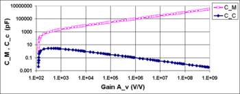
or
which provides a quadratic equation to determine an appropriate value for CC. Figure 4 shows an example using this equation. At low values of gain this example amplifier satisfies the pole-ratio condition without compensation (that is, in Figure 4 the compensation capacitor CC is small at low gain), but as gain increases, a compensation capacitance rapidly becomes necessary (that is, in Figure 4 the compensation capacitor CC increases rapidly with gain) because the necessary pole ratio increases with gain. For still larger gain, the necessary CC drops with increasing gain because the Miller amplification of CC, which increases with gain (see the Miller equation ), allows a smaller value for CC.
To provide more safety margin for design uncertainties, often Av is increased to two or three times Av on the right side of this equation. See Sansen or Huijsing and article on step responseStep responseThe step response of a system in a given initial state consists of the time evolution of its outputs when its control inputs are Heaviside step functions. In electronic engineering and control theory, step response is the time behaviour of the outputs of a general system when its inputs change from...
.
Slew rate
The above is a small-signal analysis. However, when large signals are used, the need to charge and discharge the compensation capacitor adversely affects the amplifier slew rateSlew rateIn electronics, the slew rate represents the maximum rate of change of a signal at any point in a circuit.Limitations in slew rate capability can give rise to non linear effects in electronic amplifiers...
; in particular, the response to an input ramp signal is limited by the need to charge CC.
See also
- Frequency compensationFrequency compensationIn electrical engineering, frequency compensation is a technique used in amplifiers, and especially in amplifiers employing negative feedback. It usually has two primary goals: To avoid the unintentional creation of positive feedback, which will cause the amplifier to oscillate, and to control...
- Step responseStep responseThe step response of a system in a given initial state consists of the time evolution of its outputs when its control inputs are Heaviside step functions. In electronic engineering and control theory, step response is the time behaviour of the outputs of a general system when its inputs change from...
- Miller effectMiller effectIn electronics, the Miller effect accounts for the increase in the equivalent input capacitance of an inverting voltage amplifier due to amplification of the effect of capacitance between the input and output terminals...
- Common sourceCommon sourceIn electronics, a common-source amplifier is one of three basic single-stage field-effect transistor amplifier topologies, typically used as a voltage or transconductance amplifier. The easiest way to tell if a FET is common source, common drain, or common gate is to examine where the signal...
- Bode plotBode plotA Bode plot is a graph of the transfer function of a linear, time-invariant system versus frequency, plotted with a log-frequency axis, to show the system's frequency response...
- Step response
External links
- Bode Plots in the Circuit Theory WikibookWikibooksWikibooks is a Wiki hosted by the Wikimedia Foundation for the creation of free content textbooks and annotated texts that anyone can edit....
- Bode Plots in the Control Systems WikibookWikibooksWikibooks is a Wiki hosted by the Wikimedia Foundation for the creation of free content textbooks and annotated texts that anyone can edit....
-
-
-
-
-
-
-