

Point-biserial correlation coefficient
Encyclopedia
The point biserial correlation coefficient (rpb) is a correlation coefficient
used when one variable (e.g. Y) is dichotomous
; Y can either be "naturally" dichotomous, like gender, or an artificially dichotomized variable. In most situations it is not advisable to artificially dichotomize variables. When you artificially dichotomize a variable the new dichotomous variable may be conceptualized as having an underlying continuity. If this is the case, a biserial correlation would be the more appropriate calculation.
The point-biserial correlation is mathematically equivalent to the Pearson (product moment) correlation
, that is, if we have one continuously measured variable X and a dichotomous variable Y, rXY = rpb. This can be shown by assigning two distinct numerical values to the dichotomous variable.
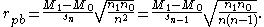
To calculate rpb, assume that the dichotomous variable Y has the two values 0 and 1. If we divide the data set into two groups, group 1 which received the value "1" on Y and group 2 which received the value "0" on Y, then the point-biserial correlation coefficient is calculated as follows: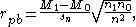
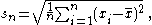
where sn is the standard deviation used when you have data for every member of the population:
M1 being the mean value on the continuous variable X for all data points in group 1, and M0 the mean value on the continuous variable X for all data points in group 2. Further, n1 is the number of data points in group 1, n0 is the number of data points in group 2 and n is the total sample size. This formula is a computational formula that has been derived from the formula for rXY in order to reduce steps in the calculation; it is easier to compute than rXY.
It is easy to show algebraically that there is an equivalent formula that uses sn−1:
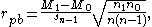
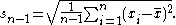
where sn−1 is the standard deviation used when you only have data for a sample of the population:
To clarify:
Glass and Hopkins' book Statistical Methods in Education and Psychology, (3rd Edition) contains a correct version of point biserial formula.
Also the square of the point biserial correlation coefficient can be written: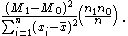
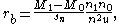
We can test the null hypothesis that the correlation is zero in the population. A little algebra shows that the usual formula for assessing the significance of a correlation coefficient, when applied to rpb, is the same as the formula for an unpaired t-test
and so

follows Student's t-distribution with (n1+n0 - 2) degrees of freedom when the null hypothesis is true.
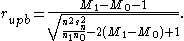
One disadvantage of the point biserial coefficient is that the further the distribution of Y is from 50/50, the more constrained will be the range of values which the coefficient can take. If X can be assumed to be normally distributed, a better descriptive index is given by the biserial coefficient
where u is the ordinate of the normal distribution with zero mean and unit variance at the point which divides the distribution into proportions n0/n and n1/n. As you might imagine, this is not the easiest thing in the world to calculate and the biserial coefficient is not widely used in practice.
A specific case of biserial correlation occurs where X is the sum of a number of dichotomous variables of which Y is one. An example of this is where X is a person's total score on a test composed of n dichotomously scored items. A statistic of interest (the discrimination index) is the correlation between a given item and the total test score. But since the latter includes the former, a measure of positive correlation is guaranteed and the statistic is biased. In this case the usual formula for the point biserial coefficient is replaced by
A slightly different version of the point biserial coefficient is the rank biserial which occurs where the variable X consists of ranks while Y is dichotomous. We could calculate the coefficient in the same way as where X is continuous but it would have the same disadvantage that the range of values it can take on becomes more constrained as the distribution of Y becomes more unequal. To get round this, we note that the coefficient will have its largest value where the smallest ranks are all opposite the 0s and the largest ranks are opposite the 1s. Its smallest value occurs where the reverse is the case. These values are respectively plus and minus (n1 + n0)/2. We can therefore use the reciprocal of this value to rescale the difference between the observed mean ranks on to the interval from plus one to minus one. The result is

where M1 and M0 are respectively the means of the ranks corresponding to the 1 and 0 scores of the dichotomous variable. This formula, which simplifies the calculation from the counting of agreements and inversions, is due to Gene V Glass (1966).
It is possible to use this to test the null hypothesis of zero correlation in the population from which the sample was drawn. If rrb is calculated as above then the smaller of

and

is distributed as Mann–Whitney U with sample sizes n1 and n0 when the null hypothesis is true.
Pearson product-moment correlation coefficient
In statistics, the Pearson product-moment correlation coefficient is a measure of the correlation between two variables X and Y, giving a value between +1 and −1 inclusive...
used when one variable (e.g. Y) is dichotomous
Dichotomy
A dichotomy is any splitting of a whole into exactly two non-overlapping parts, meaning it is a procedure in which a whole is divided into two parts...
; Y can either be "naturally" dichotomous, like gender, or an artificially dichotomized variable. In most situations it is not advisable to artificially dichotomize variables. When you artificially dichotomize a variable the new dichotomous variable may be conceptualized as having an underlying continuity. If this is the case, a biserial correlation would be the more appropriate calculation.
The point-biserial correlation is mathematically equivalent to the Pearson (product moment) correlation
Correlation
In statistics, dependence refers to any statistical relationship between two random variables or two sets of data. Correlation refers to any of a broad class of statistical relationships involving dependence....
, that is, if we have one continuously measured variable X and a dichotomous variable Y, rXY = rpb. This can be shown by assigning two distinct numerical values to the dichotomous variable.
To calculate rpb, assume that the dichotomous variable Y has the two values 0 and 1. If we divide the data set into two groups, group 1 which received the value "1" on Y and group 2 which received the value "0" on Y, then the point-biserial correlation coefficient is calculated as follows:
where sn is the standard deviation used when you have data for every member of the population:
M1 being the mean value on the continuous variable X for all data points in group 1, and M0 the mean value on the continuous variable X for all data points in group 2. Further, n1 is the number of data points in group 1, n0 is the number of data points in group 2 and n is the total sample size. This formula is a computational formula that has been derived from the formula for rXY in order to reduce steps in the calculation; it is easier to compute than rXY.
It is easy to show algebraically that there is an equivalent formula that uses sn−1:
where sn−1 is the standard deviation used when you only have data for a sample of the population:
To clarify:
Glass and Hopkins' book Statistical Methods in Education and Psychology, (3rd Edition) contains a correct version of point biserial formula.
Also the square of the point biserial correlation coefficient can be written:
We can test the null hypothesis that the correlation is zero in the population. A little algebra shows that the usual formula for assessing the significance of a correlation coefficient, when applied to rpb, is the same as the formula for an unpaired t-test
Student's t-test
A t-test is any statistical hypothesis test in which the test statistic follows a Student's t distribution if the null hypothesis is supported. It is most commonly applied when the test statistic would follow a normal distribution if the value of a scaling term in the test statistic were known...
and so
follows Student's t-distribution with (n1+n0 - 2) degrees of freedom when the null hypothesis is true.
One disadvantage of the point biserial coefficient is that the further the distribution of Y is from 50/50, the more constrained will be the range of values which the coefficient can take. If X can be assumed to be normally distributed, a better descriptive index is given by the biserial coefficient
where u is the ordinate of the normal distribution with zero mean and unit variance at the point which divides the distribution into proportions n0/n and n1/n. As you might imagine, this is not the easiest thing in the world to calculate and the biserial coefficient is not widely used in practice.
A specific case of biserial correlation occurs where X is the sum of a number of dichotomous variables of which Y is one. An example of this is where X is a person's total score on a test composed of n dichotomously scored items. A statistic of interest (the discrimination index) is the correlation between a given item and the total test score. But since the latter includes the former, a measure of positive correlation is guaranteed and the statistic is biased. In this case the usual formula for the point biserial coefficient is replaced by
A slightly different version of the point biserial coefficient is the rank biserial which occurs where the variable X consists of ranks while Y is dichotomous. We could calculate the coefficient in the same way as where X is continuous but it would have the same disadvantage that the range of values it can take on becomes more constrained as the distribution of Y becomes more unequal. To get round this, we note that the coefficient will have its largest value where the smallest ranks are all opposite the 0s and the largest ranks are opposite the 1s. Its smallest value occurs where the reverse is the case. These values are respectively plus and minus (n1 + n0)/2. We can therefore use the reciprocal of this value to rescale the difference between the observed mean ranks on to the interval from plus one to minus one. The result is
where M1 and M0 are respectively the means of the ranks corresponding to the 1 and 0 scores of the dichotomous variable. This formula, which simplifies the calculation from the counting of agreements and inversions, is due to Gene V Glass (1966).
It is possible to use this to test the null hypothesis of zero correlation in the population from which the sample was drawn. If rrb is calculated as above then the smaller of
and
is distributed as Mann–Whitney U with sample sizes n1 and n0 when the null hypothesis is true.
External links
- Point Biserial Coefficient (Keith Calkins, 2005)