Transmission line matrix method
Encyclopedia
The transmission-line matrix (TLM) method is a space and time discretising method for computation of electromagnetic fields. It is based on the analogy between the electromagnetic field and a mesh of transmission line
s. The TLM method allows the computation of complex three-dimensional electromagnetic structures and has proven to be one of the most powerful time-domain methods along with the finite difference time domain (FDTD) method.
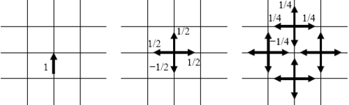 The TLM method is based on Huygens' model of wave propagation and scattering and the analogy between field propagation and transmission lines. Therefore it considers the computational domain as a mesh of transmission lines, interconnected at nodes. In the figure on the right is considered a simple example of a 2D TLM mesh with a voltage pulse of amplitude 1 V incident on the central node. This pulse will be partially reflected and transmitted according to the transmission-line theory. If we assume that each line has a characteristic impedance
  , then the incident pulse sees effectively three transmission lines in parallel with a total impedance of
  . The reflection coefficient and the transmission coefficient are given by
The energy injected into the node by the incident pulse and the total energy of the scattered pulses are correspondingly
Therefore the energy conservation law is fulfilled by the model.
The next scattering event excites the neighbouring nodes according to the principle described above. It can be seen that every node turns into a secondary source of spherical wave. These waves combine to form the overall waveform. This is in accordance with Huygens principle of light propagation.
In order to show the TLM schema we will use time and space discretisation. The time-step will be denoted with and the space discretisation intervals with
  ,
,  and
and  . The absolute time and space will therefore be
  ,
,  ,
,  ,
,  , where
  is the time instant and
  are the cell coordinates. In case
  the value
  will be used, which is the lattice constant
. In this case the following holds:
 If we consider an electromagnetic field distribution, in which the only non-zero components are
  ,
,  and
and  (i.e. a TE-mode distribution), the Maxwell's equations in Cartesian coordinates reduce to
We can combine these equations to obtain
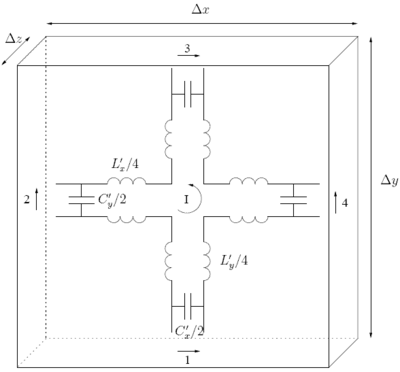
The figure on the right presents a structure, referred to as a series node. It describes a block of space dimensions ,
,  and
and  and consists of four ports.
  and
and  are the distributed inductance and capacitance of the transmission lines. It is possible to show that a series node is equivalent to a TE-wave, more precisely the mesh current I, the x-direction voltages (ports 1 and 3) and the y-direction voltages (ports 2 and 4) may be related to the field components
  ,
,  and
and  . If the voltages on the ports are considered,
  , and the polarity from figure holds, than the following is valid
where .
.
and dividing both sides by
Since and substituting
  gives
gives
This reduces to the Maxwell's equation when .
.
Similarly, using the conditions across the capacitor on ports 1 and 4, it can be shown that the corresponding to the other two Maxwell equations are the following:
Having these results it is possible to compute the scattering matrix of a shunt node. The incident voltage pulse on port 1 at time-step k is denoted as . Replacing the four line segments from figure with their Thevenin equivalent it is possible to show that the following equation for the reflected voltage pulse holds:
If all incident waves are summarised in one vector as well as all reflected waves, this equation may be written down for all ports in matrix form:
where and
and  are the incident and the reflected pulse amplitude vectors.
For a series node the scattering matrix S has the following form
Transmission line
In communications and electronic engineering, a transmission line is a specialized cable designed to carry alternating current of radio frequency, that is, currents with a frequency high enough that its wave nature must be taken into account...
s. The TLM method allows the computation of complex three-dimensional electromagnetic structures and has proven to be one of the most powerful time-domain methods along with the finite difference time domain (FDTD) method.
Basic principle
, then the incident pulse sees effectively three transmission lines in parallel with a total impedance of . The reflection coefficient and the transmission coefficient are given by
The energy injected into the node by the incident pulse and the total energy of the scattered pulses are correspondingly


Therefore the energy conservation law is fulfilled by the model.
The next scattering event excites the neighbouring nodes according to the principle described above. It can be seen that every node turns into a secondary source of spherical wave. These waves combine to form the overall waveform. This is in accordance with Huygens principle of light propagation.
In order to show the TLM schema we will use time and space discretisation. The time-step will be denoted with
and the space discretisation intervals with , and . The absolute time and space will therefore be , , , , where is the time instant and are the cell coordinates. In case the value will be used, which is the lattice constantLattice constant
The lattice constant [or lattice parameter] refers to the constant distance between unit cells in a crystal lattice. Lattices in three dimensions generally have three lattice constants, referred to as a, b, and c. However, in the special case of cubic crystal structures, all of the constants are...
. In this case the following holds:

The scattering matrix of an 2D TLM node
, and (i.e. a TE-mode distribution), the Maxwell's equations in Cartesian coordinates reduce to

We can combine these equations to obtain
The figure on the right presents a structure, referred to as a series node. It describes a block of space dimensions
, and and consists of four ports. and are the distributed inductance and capacitance of the transmission lines. It is possible to show that a series node is equivalent to a TE-wave, more precisely the mesh current I, the x-direction voltages (ports 1 and 3) and the y-direction voltages (ports 2 and 4) may be related to the field components , and . If the voltages on the ports are considered, , and the polarity from figure holds, than the following is valid
where
.

and dividing both sides by

Since
and substituting gives
This reduces to the Maxwell's equation when
.Similarly, using the conditions across the capacitor on ports 1 and 4, it can be shown that the corresponding to the other two Maxwell equations are the following:


Having these results it is possible to compute the scattering matrix of a shunt node. The incident voltage pulse on port 1 at time-step k is denoted as
. Replacing the four line segments from figure with their Thevenin equivalent it is possible to show that the following equation for the reflected voltage pulse holds:
If all incident waves are summarised in one vector as well as all reflected waves, this equation may be written down for all ports in matrix form:

where
and are the incident and the reflected pulse amplitude vectors.For a series node the scattering matrix S has the following form
-
Connection between TLM nodes
In order to describe the connection between adjacent nodes the mesh of series nodes look at the figure on the right. As the incident pulse in timestep k+1 on a node is the scattered pulse from an adjacent node in timestep k the following connection equations are derived: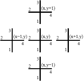
By modifying the scattering matrix inhomogeneous and lossy materials can be modelled. By adjusting the connection equations it is possible to simulate different boundaries.
The shunt TLM node
Apart from the series node, described above there is also the shunt TLM node, which represents a TM-mode field distribution. The only non-zero components of such wave are ,
,  , and
, and  . With similar considerations as for the series node the scattering matrix of the shunt node may be derived.
3D TLM models
Most problems in electromagnetics require a three-dimensional computing. As we have structures, that describe TE and TM-field distributions, intuitively it seem possible to provide a combination of shunt and series nodes, which will provide a full description of the electromagnetic field. Such attempts have been made, but they proved not very useful because of the complexity of the resulting structures. Using the normal analogy, presented above, leads to calculation of the different field components at physically separated points. This causes difficulties in simple and efficient boundary definition. A solution to these problems was provided by Johns in 1987, when he proposed the structure, known as the symmetrical condensed node (SCN), presented in the figure. It consists of 12 ports, because two field polarisations are to be assigned to each of the 6 sides of a mesh cell.
The topology of the SCN can not be analysed using Thevenin equivalent circuits. More general energy and charge conservation principles are to be used.
The electric and the magnetic fields on the sides of the SCN node number (l,m,n) at time instant k may be summarised in 12-dimensional vectors
They can be linked with the incident and scattered amplitude vectors via
where is the field impedance,
  is the vector of the amplitudes of the incident waves to the node, and
  is the vector of the scattered amplitudes. The relation between the incident and scattered waves is given with the matrix equation
The scattering matrix S may be calculated. For the symmetrical condensed node with ports defined as in the figure the following result is obtained
-
where the following matrix was used
-
The connection between different SCNs is done in the same manner as for the 2D nodes.
-
-