
Niche apportionment models
Encyclopedia
Mechanistic models for niche apportionment are biological models used to explain relative species abundance
distributions. These models describe how species break up resource
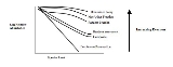
pool in multi-dimensional space, determining the distribution of abundances of individuals among species. The relative abundances of species are usually expressed as a Whittaker plot (figure 1), or rank abundance plot, where species are ranked by number of individuals on the x-axis, plotted against the log relative abundance of each species on the y-axis. The relative abundance can be measured as the relative number of individuals within species or the relative biomass of individuals within species.
distributions. MacArthur (1957, 1961), was one of the earliest to express dissatisfaction with purely statistical models, presenting instead 3 mechanistic niche apportionment models. MacArthur believed that ecological niches within a resource pool could be broken up like a stick, with each piece of the stick representing niches occupied in the community. With contributions from Sugihara (1980), Tokeshi (1990, 1993. 1996) expanded upon the Broken Stick model, when he generated roughly 7 mechanistic niche apportionment models. These mechanistic models provide a useful starting point for describing the species composition of communities.
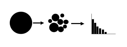
These models describe how species that draw from the same resource pool (e.g. a guild (ecology)
) partition their niche. The resource pool is broken either sequentially or simultaneously, and the two components of the process of fragmentation of the niche include which fragment is chosen and the size of the resulting fragment (Figure 2).
Niche apportionment models have been used in the primary literature to explain, and describe changes in the relative abundance distributions of a diverse array of taxa including, freshwater insects, fish, bryophytes beetles, hymenopteran parasites, plankton assemblages and salt marsh grass.
 The mechanistic models that describe these plots work under the assumption that rank abundance plots are based on a rigorous estimate of the abundances of individuals within species and that these measures represent the actual species abundance distribution. Furthermore, whether using the number of individuals as the abundance measure or the biomass of individuals, these models assume that this quantity is directly proportional to the size of the niche occupied by an organism (add a direct sentence explaining size structure and biomass and thus energy use by each individual). One suggestion is that abundance measured as the numbers of individuals, may exhibit lower variances than those using biomass
. Thus, some studies using abundance as a proxy for niche allocation may overestimate the evenness of a community
. This happens because there is not a clear distinction of the relationship between body
size
, abundance (ecology)
, and resource
use. Often studies fail to incorporate size structure or biomass estimates into measures of actual abundance, and these measure can create a higher variance around the niche apportionment models than abundance measured strictly as the number of individuals..
, including some taxonomic groupings, and specific functional groupings..
The Geometric (k=0.75)
, in that different niche apportionment models fit different functional groups of the data. Another example by Higgins and Strauss (2008), modeling fish assemblages, found that fish communities from different habitats and with different species compositions conform to different niche apportionment models, thus the entire species assemblage was a combination of models in different regions of the species range.
For many years the fit of niche apportionment models was conducted by eye and graphs of the models were compared with empirical data. More recently statistical tests of the fit of niche apportionment models to empirical data have been developed . The later method (Etienne and Ollf 2005) uses a Bayesian simulation of the models to test their fit to empirical data. The former method, which is still commonly used, simulates the expected relative abundances, from a normal distribution, of each model given the same number of species as the empirical data. Each model is simulated multiple times, and mean and standard deviation can be calculated to assign confidence intervals around each relative abundance distribution. The confidence around each rank can be tested against empirical data for each model to determine model fit. The confidence intervals are calculated as follows. For more information on the simulation of niche apportionment models the website http://www.entu.cas/png/PowerNiche, which explains the program Power Niche .

r=confidence limit of simulated data
σ=standard deviation of simulated data
n=number of replicates of empirical sample
Relative species abundance
Relative species abundance is a component of biodiversity and refers to how common or rare a species is relative to other species in a defined location or community...
distributions. These models describe how species break up resource
Resource
A resource is a source or supply from which benefit is produced, typically of limited availability.Resource may also refer to:* Resource , substances or objects required by a biological organism for normal maintenance, growth, and reproduction...
pool in multi-dimensional space, determining the distribution of abundances of individuals among species. The relative abundances of species are usually expressed as a Whittaker plot (figure 1), or rank abundance plot, where species are ranked by number of individuals on the x-axis, plotted against the log relative abundance of each species on the y-axis. The relative abundance can be measured as the relative number of individuals within species or the relative biomass of individuals within species.
History
Niche apportionment models were developed because ecologists sought biological explanations for relative species abundanceRelative species abundance
Relative species abundance is a component of biodiversity and refers to how common or rare a species is relative to other species in a defined location or community...
distributions. MacArthur (1957, 1961), was one of the earliest to express dissatisfaction with purely statistical models, presenting instead 3 mechanistic niche apportionment models. MacArthur believed that ecological niches within a resource pool could be broken up like a stick, with each piece of the stick representing niches occupied in the community. With contributions from Sugihara (1980), Tokeshi (1990, 1993. 1996) expanded upon the Broken Stick model, when he generated roughly 7 mechanistic niche apportionment models. These mechanistic models provide a useful starting point for describing the species composition of communities.
Description
A niche apportionment model can be used in situations where one resource pool is either sequentially or simultaneously broken up into smaller niches by colonizing species or by speciation (clarification on resource use: species within a guild use same resources, while species within a community may not).These models describe how species that draw from the same resource pool (e.g. a guild (ecology)
Guild (ecology)
A guild is any group of species that exploit the same resources, often in related ways. As can be seen from the list of examples below, it does not follow that the species within a guild occupy the same, or even similar, ecological niches...
) partition their niche. The resource pool is broken either sequentially or simultaneously, and the two components of the process of fragmentation of the niche include which fragment is chosen and the size of the resulting fragment (Figure 2).
Niche apportionment models have been used in the primary literature to explain, and describe changes in the relative abundance distributions of a diverse array of taxa including, freshwater insects, fish, bryophytes beetles, hymenopteran parasites, plankton assemblages and salt marsh grass.
Assumptions
Biomass
Biomass, as a renewable energy source, is biological material from living, or recently living organisms. As an energy source, biomass can either be used directly, or converted into other energy products such as biofuel....
. Thus, some studies using abundance as a proxy for niche allocation may overestimate the evenness of a community
Community
The term community has two distinct meanings:*a group of interacting people, possibly living in close proximity, and often refers to a group that shares some common values, and is attributed with social cohesion within a shared geographical location, generally in social units larger than a household...
. This happens because there is not a clear distinction of the relationship between body
Body
With regard to living things, a body is the physical body of an individual. "Body" often is used in connection with appearance, health issues and death...
size
Size
The word size may refer to how big something is. In particular:* Measurement, the process or the result of determining the magnitude of a quantity, such as length or mass, relative to a unit of measurement, such as a meter or a kilogram...
, abundance (ecology)
Abundance (ecology)
Abundance is an ecological concept referring to the relative representation of a species in a particular ecosystem. It is usually measured as the large number of individuals found per sample...
, and resource
Resource
A resource is a source or supply from which benefit is produced, typically of limited availability.Resource may also refer to:* Resource , substances or objects required by a biological organism for normal maintenance, growth, and reproduction...
use. Often studies fail to incorporate size structure or biomass estimates into measures of actual abundance, and these measure can create a higher variance around the niche apportionment models than abundance measured strictly as the number of individuals..
Tokeshi's mechanistic models of niche apportionment
Seven mechanistic models that describe niche apportionment are described below. The models are presented in the order of increasing evenness, from least even, the Dominance Pre-emption model to the most even the Dominance Decay and MacArthur Fraction models. Figure 1 is a graphical representation of these models on a Whittaker rank abundance plot.Dominance preemption
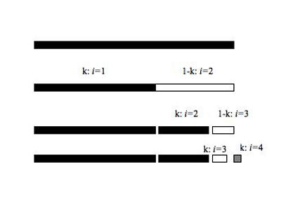
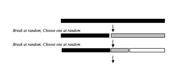
This model describes a situation where after initial colonization (or speciation) each new species pre-empts more than 50% the smallest remaining niche. In a Dominance preemption model of niche apportionment the species colonize random portion between 50 and 100% of the smallest remaining niche, making this model stochastic in nature. A closely related model, the Geometric Series, is a deterministic version of the Dominance pre-emption model, wherein the percentage of remaining niche space that the new species occupies (k) is always the same. In fact, the dominance pre-emption and geometric series models are conceptually similar and will produce the same relative abundance distribution when the proportion of the smaller niche filled is always 0.75. The dominance pre-emption model is the best fit to the relative abundance distributions of some stream fish communities in TexasTexas
Texas is the second largest U.S. state by both area and population, and the largest state by area in the contiguous United States.The name, based on the Caddo word "Tejas" meaning "friends" or "allies", was applied by the Spanish to the Caddo themselves and to the region of their settlement in...
, including some taxonomic groupings, and specific functional groupings..
The Geometric (k=0.75)
Random assortment
In the random assortment model the resource pool is divided at random among simultaneously or sequentially colonizing species. This pattern could arise because the abundance measure does not scale with the amount of niche occupied by a species or because temporal-variation in species abundance or niche breadth causes discontinuity in niche apportionment over time and thus species appear to have no relationship between extent of occupancy and their niche. Tokeshi (1993) explained that this model, in many ways, is similar to Caswell’s neutral theory of biodiversity, mainly because species appear to act independently of each other.Random fraction
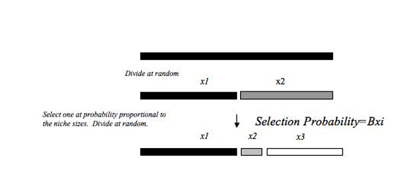
The random fraction model describes a process where niche size is chosen at random by sequentially colonizing species. The initial species chooses a random portion of the total niche and subsequent colonizing species also choose a random portion of the total niche and divide it randomly until all species have colonized. Tokeshi (1990) found this model to be compatible with some epiphytic Chiromonid shrimp communities, and more recently it has been used to explain the relative abundance distributions of phytoplankton communities, salt meadow vegetation, some communities of insects in the order Diptera, some ground beetle communities, functional and taxonomic groupings of stream fish in Texas bio-regions, and ichneumonid parasitoids. A similar model was developed by Sugihara in an attempt to provide a biological explanation for the log normal distribution of Preston (1948). Sugihara’s (1980) Fixed Division Model was similar to the random fraction model, but the randomness of the model is drawn from a triangular distribution with a mean of 0.75 rather that a normal distribution with a mean of 0.5 used in the random fraction. Sugihara used a triangular distribution to draw the random variables because the randomness of some natural populations matches a triangular distribution with a mean of 0.75.Power fraction
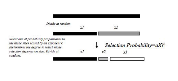
This model can explain a relative abundance distribution when the probability of colonization an existing niche in a resource pool is positively related to the size of that niche (measured as abundance, biomass etc.). The probability with which a portion of the niche colonized is dependent on the relative sizes of the established niches, and is scaled by an exponent k. k can take a value between 0 and 1 and if k>0 there is always a slightly higher probably that the larger niche will be colonized. This model is toted as being more biologically realistic because one can imagine many cases where the species with the larger proportion of resources is more likely to be invaded because that niche has more resource space, and thus more opportunity for acquisition. The random fraction model of niche apportionment is an extreme of the power fraction model where k=0, and the other extreme of the power fraction, when k=1 resembles the MacArthur Fraction model where the probability of colonization is directly proportion to niche size.MacArthur fraction
This model requires that the initial niche is broken at random and the successive niches are chosen with a probability proportional to their size. In this model the largest niche always has a greater probability of being broken relative to the smaller niches in the resource pool. This model can lead to a more even distribution where larger niches are more likely to be broken facilitating co-existence between species in equivalent sized niches. The basis for the MacArthur Fraction model is the Broken Stick, developed by MacArthur (1957). These models produce similar results, but one of the main conceptual differences is that niches are filled simultaneously in Broken Stick model rather than sequentially as in the MacArthur Fraction. Tokeshi (1993) argues that sequentially invading a resource pool is more biologically realistic than simultaneously breaking the niche space. When the abundance of fish from all bio-regions in Texas were combined the distribution resembled the broken stick model of niche apportionment, suggesting a relatively even distribution of freshwater fish species in Texas .Dominance decay
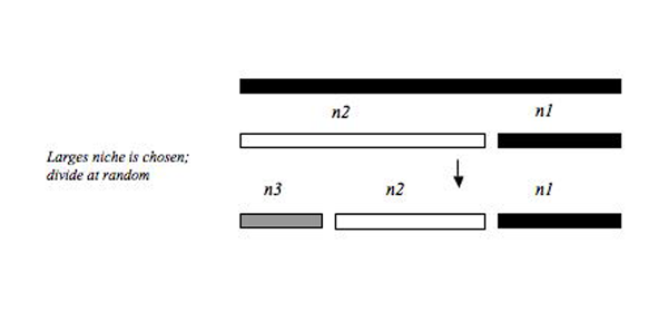
This model can be thought of as the inverse to the Dominance pre-emption model. First, the initial resource pool is colonized randomly and the remaining, subsequent colonizers always colonize the largest niche, whether or not it is already colonized. This model generates the most even community relative to the niche apportionment models described above because the largest niche is always broken into two smaller fragments that are more likely to be equivalent to the size of the smaller niche that was not broken. Communities of this “level” of evenness seem to be rare in natural systems. However, one such community includes the relative abundance distribution of filter feeders in one site within the River Danube in Austria .Composite
A composite model exists when a combination of niche apportionment models are acting in different portions of the resource pool. Fesl (2002). shows how a composite model might appear in a study of freshwater DipteraDiptera
Diptera , or true flies, is the order of insects possessing only a single pair of wings on the mesothorax; the metathorax bears a pair of drumstick like structures called the halteres, the remnants of the hind wings. It is a large order, containing an estimated 240,000 species, although under half...
, in that different niche apportionment models fit different functional groups of the data. Another example by Higgins and Strauss (2008), modeling fish assemblages, found that fish communities from different habitats and with different species compositions conform to different niche apportionment models, thus the entire species assemblage was a combination of models in different regions of the species range.
Fitting mechanistic models of niche apportionment to empirical data
Mechanistic models of niche apportionment are intended to describe communities. Researchers have used these models in many ways to investigate the temporal and geographic trends in species abundance.For many years the fit of niche apportionment models was conducted by eye and graphs of the models were compared with empirical data. More recently statistical tests of the fit of niche apportionment models to empirical data have been developed . The later method (Etienne and Ollf 2005) uses a Bayesian simulation of the models to test their fit to empirical data. The former method, which is still commonly used, simulates the expected relative abundances, from a normal distribution, of each model given the same number of species as the empirical data. Each model is simulated multiple times, and mean and standard deviation can be calculated to assign confidence intervals around each relative abundance distribution. The confidence around each rank can be tested against empirical data for each model to determine model fit. The confidence intervals are calculated as follows. For more information on the simulation of niche apportionment models the website http://www.entu.cas/png/PowerNiche, which explains the program Power Niche .
r=confidence limit of simulated data
σ=standard deviation of simulated data
n=number of replicates of empirical sample