

Method of conditional probabilities
Encyclopedia
In mathematics
and computer science
, the probabilistic method
is used to prove the existence of mathematical objects with desired combinatorial properties. The proofs are probabilistic — they work by showing that a random object, chosen from some probability distribution, has the desired properties with positive probability. Consequently, they are nonconstructive — they don't explicitly describe an efficient method for computing the desired objects.
The method of conditional probabilities
,
,
converts such a proof, in a "very precise sense",
into an efficient deterministic algorithm
,
one that is guaranteed to compute an object with the desired properties.
That is, the method derandomizes the proof.
The basic idea is to replace each random choice in a random experiment
by a deterministic choice, so as to keep the conditional probability of failure,
given the choices so far, below 1.
The method is particularly relevant in the context of randomized rounding
(which uses the probabilistic method to design approximation algorithm
s).
When applying the method of conditional probabilities,
the technical term pessimistic estimator refers to a quantity used
in place of the true conditional probability (or conditional expectation)
underlying the proof.
(Raghavan is discussing the method in the context of randomized rounding
,
but it works with the probabilistic method in general.)
To apply the method to a probabilistic proof, the randomly chosen object in the proof
must be choosable by a random experiment that consists of a sequence of "small" random choices.
Here is a trivial example to illustrate the principle.
In this example the random experiment consists of flipping three fair coins.
The experiment is illustrated by the rooted tree in the diagram to the right.
There are eight outcomes, each corresponding to a leaf in the tree.
A trial of the random experiment corresponds to taking a random walk
from the root (the top node in the tree, where no coins have been flipped) to a leaf.
The successful outcomes are those in which at least two coins came up tails.
The interior nodes in the tree correspond to partially determined outcomes,
where only 0, 1, or 2 of the coins have been flipped so far.
To apply the method of conditional probabilities,
one focuses on the conditional probability of failure,
given the choices so far as the experiment proceeds step by step.
In the diagram, each node is labeled with this conditional probability.
(For example, if only the first coin has been flipped,
and it comes up tails, that corresponds to the second child of the root.
Conditioned on that partial state, the probability of failure is 0.25.)
The method of conditional probabilities replaces the random root-to-leaf walk
in the random experiment by a deterministic root-to-leaf walk,
where each step is chosen to inductively maintain the following invariant:
In this way, it is guaranteed to arrive at a leaf with label 0, that is, a successful outcome.
The invariant holds initially (at the root), because the original proof
showed that the (unconditioned) probability of failure is less than 1.
The conditional probability at any interior node
is the average of the conditional probabilities of its children.
The latter property is important because it implies that
any interior node whose conditional probability is less than 1 has at least one child whose conditional probability is less than 1.
Thus, from any interior node, one can always choose some child
to walk to so as to maintain the invariant.
Since the invariant holds at the end, when the walk arrives at a leaf
and all choices have been determined,
the outcome reached in this way must be a successful one.
the goal is to be able to implement the resulting deterministic process
by a reasonably efficient algorithm
(formally, one taking time polynomial in the input size),
even though typically the number of possible outcomes is huge (exponentially large).
(E.g., consider the example above, but extended to flips for large
  .)
.)
In the ideal case, given a partial state (a node in the tree),
the conditional probability of failure (the label on the node)
can be efficiently and exactly computed.
(The example above is like this.)
If this is so, then the algorithm can select the next node to go to
by computing the conditional probabilities at each of the children
of the current node, then moving to any child whose conditional
probability is less than 1.
As discussed above, there is guaranteed to be such a node.
Unfortunately, in most applications,
the conditional probability of failure is not easy to compute efficiently.
There are two standard and related techniques for dealing with this:
In this case, to keep the conditional probability of failure below 1, it suffices to keep the conditional expectation of below (or above) the threshold. To do this, instead of computing the conditional probability of failure, the algorithm computes the conditional expectation of
  and proceeds accordingly: at each interior node, there is some child whose conditional expectation is at most (at least) the node's conditional expectation; the algorithm moves from the current node to such a child, thus keeping the conditional expectation below (above) the threshold.
 ,
,
the Max cut problem is to color each vertex of the graph with one of two colors (say black or white)
so as to maximize the number of edges whose endpoints have different colors.
(Say such an edge is cut.)
Lemma: In any graph , at least
  edges can be cut.
By calculation, for any edge e in , the probability that it is cut is 1/2.
Thus, by linearity of expectation, the expected number of edges cut is .
.
Thus, there exists a coloring that cuts at least edges. QED
first model the random experiment as a sequence of small random steps.
In this case it is natural to consider each step to be the choice of color
for a particular vertex (so there are steps).
Next, replace the random choice at each step by a deterministic choice,
so as to keep the conditional probability of failure, given the vertices colored so far,
below 1. (Here failure means that finally fewer than edges are cut.)
In this case, the conditional probability of failure is not easy to calculate
(indeed the original proof did not calculate the probability of failure directly).
Instead, the proof worked by showing that the expected number
of cut edges was at least .
.
Let random variable be the number of edges cut.
To keep the conditional probability of failure below 1,
it suffices to keep the conditional expectation of
at or above the threshold .
.
(This is because as long as the conditional expectation
of is at least
  ,
,
there must be some still-reachable outcome where is at least
  ,
,
so the conditional probability of reaching such an outcome is positive.)
To keep the conditional expectation of at
at  or above,
the algorithm will, at each step, color the vertex under consideration
so as to maximize the resulting conditional expectation of .
.
This suffices, because there must be some child whose conditional expectation is
at least the current state's conditional expectation
(and thus at least ).
).
Given that some of the vertices are colored already,
what is this conditional expectation?
Following the logic of the original proof,
the conditional expectation of the number of cut edges is
This is guaranteed to keep the conditional expectation at or above,
and so is guaranteed to keep the conditional probability of failure below 1,
which in turn guarantees a successful outcome.
By calculation, the algorithm simplifies to the following:
1. For each vertex in
in  (in any order):
2. Consider the already-colored neighboring vertices of .
.
3. If more of these are black then white, then color white.
4. Otherwise, color black.
Because of its derivation, this deterministic algorithm is guaranteed to cut at least half the edges of the given graph.
(This makes it a 0.5-approximation algorithm for Max-cut.)
is the following:
 :
:
1. Initialize to be the empty set.
2. For each vertex in
in  in random order:
3. If no neighbors of are in
  , add
, add  to
to 
4. Return .
.
Clearly the process computes an independent set.
Any vertex that is considered before all of its neighbors will be added to
  .
.
Thus, letting denote the degree of
  ,
,
the probability that is added to
  is at least
  .
.
By linearity of expectation, the expected size of is at least
(The inequality above follows because
 is convex
in ,
,
so the left-hand side is minimized,
subject to the sum of the degrees being fixed at ,
,
when each .) QED
 steps.
Each step considers some not-yet considered vertex
and adds to
to  if none of its neighbors have yet been added.
Let random variable be the number of vertices added to
  .
.
The proof shows that ≥
≥  .
.
We will replace each random step by a deterministic step
that keeps the conditional expectation of at or above
  .
.
This will ensure a successful outcome, that is,
one in which the independent set has size at least
  ,
,
realizing the bound in Turan's theorem.
Given that the first t steps have been taken,
let denote the vertices added so far.
Let denote those vertices that have not yet been considered,
and that have no neighbors in .
.
Given the first t steps,
following the reasoning in the original proof,
any given vertex in
in  has conditional probability
at least of being added to
  ,
,
so the conditional expectation of is at least
Let denote the above quantity,
which is called a pessimistic estimator for the conditional expectation.
The proof showed that the pessimistic estimator is initially at least .
.
(That is, ≥
≥  .)
.)
The algorithm will make each choice to keep the pessimistic estimator from decreasing,
that is, so that ≥
≥  for each
  .
.
Since the pessimistic estimator is a lower bound on the conditional expectation,
this will ensure that the conditional expectation stays above ,
,
which in turn will ensure that the conditional probability of failure stays below 1.
Let be the vertex considered by the algorithm in the next (
 st) step.
If already has a neighbor in
  ,
,
then is not added to
  and
and
(by inspection of ),
),
the pessimistic estimator is unchanged.
If does not have a neighbor in
  ,
,
then is added to
  .
.
By calculation, if is chosen randomly from the remaining vertices,
the expected increase in the pessimistic estimator is non-negative.
[The calculation: Conditioned on choosing a vertex in ,
,
the probability that a given term is dropped from the sum
in the pessimistic estimator is at most ,
,
so the expected decrease in each term in the sum is at most .
.
There are terms in the sum.
Thus, the expected decrease in the sum is at most 1.
Meanwhile, the size of increases by 1.]
Thus, there must exist some choice of that keeps the pessimistic estimator from decreasing.
 to maximize the resulting pessimistic estimator.
By the previous considerations, this keeps the pessimistic estimator from decreasing
and guarantees a successful outcome.
Below, denotes the neighbors of
  in
in 
(that is, neighbors of that are neither in
  nor have a neighbor in
  ).
).
1. Initialize to be the empty set.
2. While there exists a not-yet-considered vertex with no neighbor in
  :
:
3. Add such a vertex to
to  where
where  minimizes
  .
.
4. Return .
.
it suffices if the algorithm keeps the pessimistic estimator from decreasing (or increasing, as appropriate).
The algorithm does not necessarily have to maximize (or minimize) the pessimistic estimator.
This gives some flexibility in deriving the algorithm.
The next two algorithms illustrate this.
1. Initialize to be the empty set.
2. While there exists a vertex in the graph with no neighbor in
  :
:
3. Add such a vertex to
to  , where
  minimizes
  (the initial degree of
  ).
).
4. Return .
.
1. Initialize to be the empty set.
2. While the remaining graph is not empty:
3. Add a vertex to
to  , where
  has minimum degree in the remaining graph.
4. Delete and all of
  's neighbors from the graph.
5. Return .
.
Each algorithm is analyzed with the same pessimistic estimator as before.
With each step of either algorithm, the net increase in the pessimistic estimator is
where denotes the neighbors of
  in the remaining graph
(that is, in ).
).
For the first algorithm, the net increase is non-negative because, by the choice of ,
, ,
,
where is the degree of
  in the original graph.
For the second algorithm, the net increase is non-negative because, by the choice of ,
, ,
,
where is the degree of
  in the remaining graph.
Mathematics
Mathematics is the study of quantity, space, structure, and change. Mathematicians seek out patterns and formulate new conjectures. Mathematicians resolve the truth or falsity of conjectures by mathematical proofs, which are arguments sufficient to convince other mathematicians of their validity...
and computer science
Computer science
Computer science or computing science is the study of the theoretical foundations of information and computation and of practical techniques for their implementation and application in computer systems...
, the probabilistic method
Probabilistic method
The probabilistic method is a nonconstructive method, primarily used in combinatorics and pioneered by Paul Erdős, for proving the existence of a prescribed kind of mathematical object. It works by showing that if one randomly chooses objects from a specified class, the probability that the...
is used to prove the existence of mathematical objects with desired combinatorial properties. The proofs are probabilistic — they work by showing that a random object, chosen from some probability distribution, has the desired properties with positive probability. Consequently, they are nonconstructive — they don't explicitly describe an efficient method for computing the desired objects.
The method of conditional probabilities
,
,
converts such a proof, in a "very precise sense",
into an efficient deterministic algorithm
Deterministic algorithm
In computer science, a deterministic algorithm is an algorithm which, in informal terms, behaves predictably. Given a particular input, it will always produce the same output, and the underlying machine will always pass through the same sequence of states...
,
one that is guaranteed to compute an object with the desired properties.
That is, the method derandomizes the proof.
The basic idea is to replace each random choice in a random experiment
by a deterministic choice, so as to keep the conditional probability of failure,
given the choices so far, below 1.
The method is particularly relevant in the context of randomized rounding
Randomized rounding
Within computer science and operations research,many combinatorial optimization problems are computationally intractable to solve exactly ....
(which uses the probabilistic method to design approximation algorithm
Approximation algorithm
In computer science and operations research, approximation algorithms are algorithms used to find approximate solutions to optimization problems. Approximation algorithms are often associated with NP-hard problems; since it is unlikely that there can ever be efficient polynomial time exact...
s).
When applying the method of conditional probabilities,
the technical term pessimistic estimator refers to a quantity used
in place of the true conditional probability (or conditional expectation)
underlying the proof.
Overview
gives this description:- We first show the existence of a provably good approximate solution using the probabilistic methodProbabilistic methodThe probabilistic method is a nonconstructive method, primarily used in combinatorics and pioneered by Paul Erdős, for proving the existence of a prescribed kind of mathematical object. It works by showing that if one randomly chooses objects from a specified class, the probability that the...
... [We then] show that the probabilistic existence proof can be converted, in a very precise sense, into a deterministic approximation algorithm.
(Raghavan is discussing the method in the context of randomized rounding
Randomized rounding
Within computer science and operations research,many combinatorial optimization problems are computationally intractable to solve exactly ....
,
but it works with the probabilistic method in general.)
To apply the method to a probabilistic proof, the randomly chosen object in the proof
must be choosable by a random experiment that consists of a sequence of "small" random choices.
Here is a trivial example to illustrate the principle.
- Lemma: It is possible to flip three coins so that the number of tails is at least 2.
- Probabilistic proof. If the three coins are flipped randomly, the expected number of tails is 1.5. Thus, there must be some outcome (way of flipping the coins) so that the number of tails is at least 1.5. Since the number of tails is an integer, in such an outcome there are at least 2 tails. QED
In this example the random experiment consists of flipping three fair coins.
The experiment is illustrated by the rooted tree in the diagram to the right.
There are eight outcomes, each corresponding to a leaf in the tree.
A trial of the random experiment corresponds to taking a random walk
from the root (the top node in the tree, where no coins have been flipped) to a leaf.
The successful outcomes are those in which at least two coins came up tails.
The interior nodes in the tree correspond to partially determined outcomes,
where only 0, 1, or 2 of the coins have been flipped so far.
To apply the method of conditional probabilities,
one focuses on the conditional probability of failure,
given the choices so far as the experiment proceeds step by step.
In the diagram, each node is labeled with this conditional probability.
(For example, if only the first coin has been flipped,
and it comes up tails, that corresponds to the second child of the root.
Conditioned on that partial state, the probability of failure is 0.25.)
The method of conditional probabilities replaces the random root-to-leaf walk
in the random experiment by a deterministic root-to-leaf walk,
where each step is chosen to inductively maintain the following invariant:
-
- the conditional probability of failure, given the current state, is less than 1.
In this way, it is guaranteed to arrive at a leaf with label 0, that is, a successful outcome.
The invariant holds initially (at the root), because the original proof
showed that the (unconditioned) probability of failure is less than 1.
The conditional probability at any interior node
is the average of the conditional probabilities of its children.
The latter property is important because it implies that
any interior node whose conditional probability is less than 1 has at least one child whose conditional probability is less than 1.
Thus, from any interior node, one can always choose some child
to walk to so as to maintain the invariant.
Since the invariant holds at the end, when the walk arrives at a leaf
and all choices have been determined,
the outcome reached in this way must be a successful one.
Efficiency
In a typical application of the method,the goal is to be able to implement the resulting deterministic process
by a reasonably efficient algorithm
(formally, one taking time polynomial in the input size),
even though typically the number of possible outcomes is huge (exponentially large).
(E.g., consider the example above, but extended to
flips for large .)In the ideal case, given a partial state (a node in the tree),
the conditional probability of failure (the label on the node)
can be efficiently and exactly computed.
(The example above is like this.)
If this is so, then the algorithm can select the next node to go to
by computing the conditional probabilities at each of the children
of the current node, then moving to any child whose conditional
probability is less than 1.
As discussed above, there is guaranteed to be such a node.
Unfortunately, in most applications,
the conditional probability of failure is not easy to compute efficiently.
There are two standard and related techniques for dealing with this:
- Using a conditional expectation: Many probabilistic proofs work as follows: they implicitly define a random variable
 , show that (i) the expectation of
  is at most (or at least) some threshold value, and (ii) in any outcome where
  is at most (at least) this threshold, the outcome is a success. Then (i) implies that there exists an outcome where
  is at most the threshold, and this and (ii) imply that there is an outcome that is a success. (In the example above,
  is the number of tails, which should be at least the threshold 1.5. In many applications,
  is the number of "bad" events (not necessarily disjoint) that occur in a given outcome, where each bad event corresponds to one way the experiment can fail, and the expected number of bad events that occur is less than 1.)
In this case, to keep the conditional probability of failure below 1, it suffices to keep the conditional expectation of
below (or above) the threshold. To do this, instead of computing the conditional probability of failure, the algorithm computes the conditional expectation of and proceeds accordingly: at each interior node, there is some child whose conditional expectation is at most (at least) the node's conditional expectation; the algorithm moves from the current node to such a child, thus keeping the conditional expectation below (above) the threshold.
- Using a pessimistic estimator: In some cases, as a proxy for the exact conditional expectation of the quantity
 , one uses an appropriately tight bound called a pessimistic estimator. The pessimistic estimator is a function of the current state. It should upper (or lower) bound the conditional expectation of
  given the current state, and it should be non-increasing (or non-decreasing) in expectation with each random step of the experiment. Typically, a good pessimistic estimator can be computed by precisely deconstructing the logic of the original proof.
Example using conditional expectations
This example demonstrates the method of conditional probabilities using a conditional expectation.Max-Cut Lemma
Given any undirected graphGraph (mathematics)
In mathematics, a graph is an abstract representation of a set of objects where some pairs of the objects are connected by links. The interconnected objects are represented by mathematical abstractions called vertices, and the links that connect some pairs of vertices are called edges...
,the Max cut problem is to color each vertex of the graph with one of two colors (say black or white)
so as to maximize the number of edges whose endpoints have different colors.
(Say such an edge is cut.)
Lemma: In any graph
, at least edges can be cut.Probabilistic proof of Max-Cut lemma
Color each vertex black or white by flipping a fair coin.By calculation, for any edge e in
, the probability that it is cut is 1/2.Thus, by linearity of expectation, the expected number of edges cut is
.Thus, there exists a coloring that cuts at least
edges. QEDThe method of conditional probabilities with conditional expectations
To apply the method of conditional probabilities,first model the random experiment as a sequence of small random steps.
In this case it is natural to consider each step to be the choice of color
for a particular vertex (so there are
steps).Next, replace the random choice at each step by a deterministic choice,
so as to keep the conditional probability of failure, given the vertices colored so far,
below 1. (Here failure means that finally fewer than
edges are cut.)In this case, the conditional probability of failure is not easy to calculate
(indeed the original proof did not calculate the probability of failure directly).
Instead, the proof worked by showing that the expected number
of cut edges was at least
.Let random variable
be the number of edges cut.To keep the conditional probability of failure below 1,
it suffices to keep the conditional expectation of
at or above the threshold
.(This is because as long as the conditional expectation
of
is at least ,there must be some still-reachable outcome where
is at least ,so the conditional probability of reaching such an outcome is positive.)
To keep the conditional expectation of
at or above,the algorithm will, at each step, color the vertex under consideration
so as to maximize the resulting conditional expectation of
.This suffices, because there must be some child whose conditional expectation is
at least the current state's conditional expectation
(and thus at least
).Given that some of the vertices are colored already,
what is this conditional expectation?
Following the logic of the original proof,
the conditional expectation of the number of cut edges is
-
- the number of edges whose endpoints are colored differently so far
- + (1/2)*(the number of edges with at least one endpoint not yet colored).
Algorithm
The algorithm colors each vertex to maximize the resulting value of the above conditional expectation.This is guaranteed to keep the conditional expectation at
or above,and so is guaranteed to keep the conditional probability of failure below 1,
which in turn guarantees a successful outcome.
By calculation, the algorithm simplifies to the following:
1. For each vertex
in (in any order):2. Consider the already-colored neighboring vertices of
.3. If more of these are black then white, then color
white.4. Otherwise, color
black.Because of its derivation, this deterministic algorithm is guaranteed to cut at least half the edges of the given graph.
(This makes it a 0.5-approximation algorithm for Max-cut.)
Example using pessimistic estimators
The next example demonstrates the use of pessimistic estimators.Turán's theorem
One way of stating Turán's theoremTurán's theorem
In graph theory, Turán's theorem is a result on the number of edges in a Kr+1-free graph.An n-vertex graph that does not contain any -vertex clique may be formed by partitioning the set of vertices into r parts of equal or nearly-equal size, and connecting two vertices by an edge whenever they...
is the following:
- Any graph
 contains an independent setIndependent set (graph theory)In graph theory, an independent set or stable set is a set of vertices in a graph, no two of which are adjacent. That is, it is a set I of vertices such that for every two vertices in I, there is no edge connecting the two. Equivalently, each edge in the graph has at most one endpoint in I...
of size at least , where
  is the average degree of the graph.
Probabilistic proof of Turan's theorem
Consider the following random process for constructing an independent set:1. Initialize
to be the empty set.2. For each vertex
in in random order:3. If no neighbors of
are in , add to 4. Return
.Clearly the process computes an independent set.
Any vertex
that is considered before all of its neighbors will be added to .Thus, letting
denote the degree of ,the probability that
is added to is at least .By linearity of expectation, the expected size of
is at least
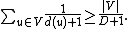
(The inequality above follows because
is convexConvex function
In mathematics, a real-valued function f defined on an interval is called convex if the graph of the function lies below the line segment joining any two points of the graph. Equivalently, a function is convex if its epigraph is a convex set...
in
,so the left-hand side is minimized,
subject to the sum of the degrees being fixed at
,when each
.) QEDThe method of conditional probabilities using pessimistic estimators
In this case, the random process has steps.Each step considers some not-yet considered vertex
and adds
to if none of its neighbors have yet been added.Let random variable
be the number of vertices added to .The proof shows that
≥ .We will replace each random step by a deterministic step
that keeps the conditional expectation of
at or above .This will ensure a successful outcome, that is,
one in which the independent set
has size at least ,realizing the bound in Turan's theorem.
Given that the first t steps have been taken,
let
denote the vertices added so far.Let
denote those vertices that have not yet been considered,and that have no neighbors in
.Given the first t steps,
following the reasoning in the original proof,
any given vertex
in has conditional probabilityat least
of being added to ,so the conditional expectation of
is at leastLet
denote the above quantity,which is called a pessimistic estimator for the conditional expectation.
The proof showed that the pessimistic estimator is initially at least
.(That is,
≥ .)The algorithm will make each choice to keep the pessimistic estimator from decreasing,
that is, so that
≥ for each .Since the pessimistic estimator is a lower bound on the conditional expectation,
this will ensure that the conditional expectation stays above
,which in turn will ensure that the conditional probability of failure stays below 1.
Let
be the vertex considered by the algorithm in the next (st) step.If
already has a neighbor in ,then
is not added to and(by inspection of
),the pessimistic estimator is unchanged.
If
does not have a neighbor in ,then
is added to .By calculation, if
is chosen randomly from the remaining vertices,the expected increase in the pessimistic estimator is non-negative.
[The calculation: Conditioned on choosing a vertex in
,the probability that a given term
is dropped from the sumin the pessimistic estimator is at most
,so the expected decrease in each term in the sum is at most
.There are
terms in the sum.Thus, the expected decrease in the sum is at most 1.
Meanwhile, the size of
increases by 1.]Thus, there must exist some choice of
that keeps the pessimistic estimator from decreasing.Algorithm maximizing the pessimistic estimator
The algorithm below chooses each vertex to maximize the resulting pessimistic estimator.By the previous considerations, this keeps the pessimistic estimator from decreasing
and guarantees a successful outcome.
Below,
denotes the neighbors of in (that is, neighbors of
that are neither in nor have a neighbor in ).1. Initialize
to be the empty set.2. While there exists a not-yet-considered vertex
with no neighbor in :3. Add such a vertex
to where minimizes .4. Return
.Algorithms that don't maximize the pessimistic estimator
For the method of conditional probabilities to work,it suffices if the algorithm keeps the pessimistic estimator from decreasing (or increasing, as appropriate).
The algorithm does not necessarily have to maximize (or minimize) the pessimistic estimator.
This gives some flexibility in deriving the algorithm.
The next two algorithms illustrate this.
1. Initialize
to be the empty set.2. While there exists a vertex
in the graph with no neighbor in :3. Add such a vertex
to , where minimizes (the initial degree of ).4. Return
.1. Initialize
to be the empty set.2. While the remaining graph is not empty:
3. Add a vertex
to , where has minimum degree in the remaining graph.4. Delete
and all of 's neighbors from the graph.5. Return
.Each algorithm is analyzed with the same pessimistic estimator as before.
With each step of either algorithm, the net increase in the pessimistic estimator is
where
denotes the neighbors of in the remaining graph(that is, in
).For the first algorithm, the net increase is non-negative because, by the choice of
,,where
is the degree of in the original graph.For the second algorithm, the net increase is non-negative because, by the choice of
,,where
is the degree of in the remaining graph.