
Beta wavelet
Encyclopedia
Continuous wavelets of compact support can be built [1], which are related to the beta distribution. The process is derived from probability distributions using blur derivative. These new wavelets have just one cycle, so they are termed unicycle wavelets. They can be viewed as a soft variety of Haar wavelet
s whose shape is fine-tuned by two parameters and
and  . Closed-form expressions for beta wavelets and scale functions as well as their spectra are derived. Their importance is due to the Central Limit Theorem
by Gnedenko&Kolmogorov applied for compactly supported signals [2].
 . It is characterised by a couple of parameters, namely
  and
and  according to:
 .
.
The normalising factor is ,
,
where is the generalised factorial function of Euler and
  is the Beta function [4].
 be a probability density of the random variable
  ,
,  i.e.
i.e.
 ,
,  and
and  .
.
Suppose that all variables are independent.
The mean and the variance of a given random variable are, respectively
 .
.
The mean and variance of are therefore
  and
and  .
.
The density of the random variable corresponding to the sum
  is given by the
Central Limit Theorem for distributions of compact support (Gnedenko and Kolmogorov) [2].
Let be distributions such that
  .
.
Let , and
, and  .
.
Without loss of generality assume that and
and  .
.
The random variable holds, as
  ,
,

where and
and 
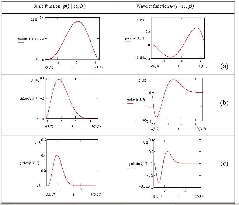
 is unimodal, the wavelet generated by
has only one-cycle (a negative half-cycle and a positive half-cycle).
The main features of beta wavelets of parameters and
and  are:
are:

The parameter is referred to as “cyclic balance”, and is defined as the ratio between the lengths of the causal and non-causal piece of the wavelet. The instant of transition
  from the first to the second half cycle is given by
The (unimodal) scale function associated with the wavelets is given by

 .
.
A closed-form expression for first-order beta wavelets can easily be derived. Within their support,

Let denote the Fourier transform pair associated with the wavelet.
This spectrum is also denoted by for short. It can be proved by applying properties of the Fourier transform that

where .
.
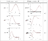
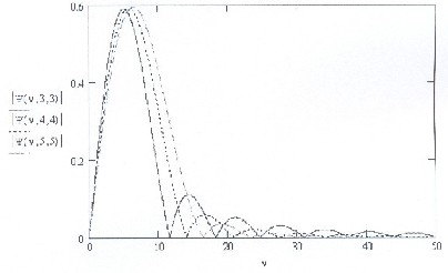
Only symmetrical cases have zeroes in the spectrum. A few asymmetric
  beta wavelets are shown in Fig. Inquisitively, they are parameter-symmetrical in the sense that they hold
Higher derivatives may also generate further beta wavelets. Higher order beta wavelets are defined by
This is henceforth referred to as an -order beta wavelet. They exist for order
  . After some algebraic handling, their closed-form expression can be found:

Haar wavelet
In mathematics, the Haar wavelet is a certain sequence of rescaled "square-shaped" functions which together form a wavelet family or basis. Wavelet analysis is similar to Fourier analysis in that it allows a target function over an interval to be represented in terms of an orthonormal function basis...
s whose shape is fine-tuned by two parameters
and . Closed-form expressions for beta wavelets and scale functions as well as their spectra are derived. Their importance is due to the Central Limit TheoremCentral limit theorem
In probability theory, the central limit theorem states conditions under which the mean of a sufficiently large number of independent random variables, each with finite mean and variance, will be approximately normally distributed. The central limit theorem has a number of variants. In its common...
by Gnedenko&Kolmogorov applied for compactly supported signals [2].
Beta distribution
The beta distribution is a continuous probability distribution defined over the interval. It is characterised by a couple of parameters, namely and according to:.The normalising factor is
,where
is the generalised factorial function of Euler and is the Beta function [4].Gnedenko-Kolmogorov central limit theorem revisited
Let be a probability density of the random variable , i.e., and .Suppose that all variables are independent.
The mean and the variance of a given random variable
are, respectively .The mean and variance of
are therefore and .The density
of the random variable corresponding to the sum is given by theCentral Limit Theorem for distributions of compact support (Gnedenko and Kolmogorov) [2].
Let
be distributions such that .Let
, and .Without loss of generality assume that
and .The random variable
holds, as , where
and Beta wavelets
Since is unimodal, the wavelet generated byhas only one-cycle (a negative half-cycle and a positive half-cycle).
The main features of beta wavelets of parameters
and are:The parameter
is referred to as “cyclic balance”, and is defined as the ratio between the lengths of the causal and non-causal piece of the wavelet. The instant of transition from the first to the second half cycle is given byThe (unimodal) scale function associated with the wavelets is given by
.A closed-form expression for first-order beta wavelets can easily be derived. Within their support,
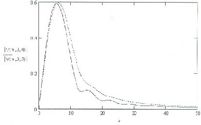
Beta wavelet spectrum
The beta wavelet spectrum can be derived in terms of the Kummer hypergeometric function [5].Let
denote the Fourier transform pair associated with the wavelet.This spectrum is also denoted by
for short. It can be proved by applying properties of the Fourier transform thatwhere
.Only symmetrical
cases have zeroes in the spectrum. A few asymmetric beta wavelets are shown in Fig. Inquisitively, they are parameter-symmetrical in the sense that they hold Higher derivatives may also generate further beta wavelets. Higher order beta wavelets are defined by
This is henceforth referred to as an
-order beta wavelet. They exist for order . After some algebraic handling, their closed-form expression can be found: