

Adaptive stepsize
Encyclopedia
Adaptive stepsize is a technique in numerical analysis
used for many problems, but mainly for integration. It can be used for both normal integration (i.e. quadrature), or the process of solving an ordinary differential equation
. This article focuses on the latter. For an explanation of adaptive stepsize in normal integration, see for example Romberg's method
.
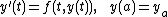
As usual, an initial value problem is stated:
Here, it is made clear that y and f can be vectors, as they will be when dealing with a system of coupled differential equations. In the rest of the article, this fact will be implicit.
Suppose we are interested in obtaining a solution at point , given a function
  , an initial time point,
  , and an initial solution
  . Of course a numerical solution will generally have an error, so we assume
  , where
  is the error.
For the sake of simplicity, the following example uses the simplest integration method, the Euler method. Note that the Euler method is almost exclusively useful for educational purposes; in practice, higher-order (Runge-Kutta) methods are used due to their superior convergence and stability properties.
Recall that the Euler method is derived from Taylor's theorem
with the intermediate value theorem and the fact that :
:
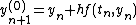
Which leads to the Euler method:
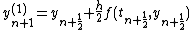
And its local truncation error
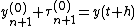
We mark this solution and its error with a . Since
  is not known to us in the general case (it depends on the derivatives of
  ), in order to say something useful about the error, a second solution should be created, using a stepsize that is smaller. For example half the original stepsize. Note that we have to apply Euler's method twice now, meaning we get two times the local error (in the worst case). Our new, and presumably more accurate solution is marked with a
  .
.
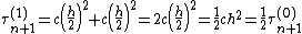
Here, we assume error factor is constant over the interval
  . In reality its rate of change is proportional to
  . Subtracting solutions gives the error estimate:
This local error estimate is third order accurate.
The local error estimate can be used to decide how stepsize should be modified to achieve the desired accuracy. For example, if a local tolerance of
  is allowed, we could let h evolve like:
The is a safety factor to ensure success on the next try. This should, in principle give an error of about
  in the next try. If
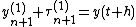
  , we consider the step successful, and the error estimate is used to improve the solution:
This solution is actually third order accurate in the local scope (second order in the global scope), but since there is no error estimate for it, this doesn't help in reducing the number of steps. This technique is called Richardson extrapolation
.
Beginning with an initial stepsize of , this theory facilitates our controllable integration of the ODE from point
  to
to  , using an optimal number of steps given a local error tolerance.
Similar methods can be developed for higher order methods, such as the Runge-Kutta 4th order method. Also, a global error tolerance can be achieved by scaling the local error to global scope. However, you might end up with a stepsize that is prohibitively small, especially using this Euler based method.
If you are interested in adaptive stepsize methods that use a so called 'embedded' error estimate, see Fehlberg, Cash-Karp and Dormand-Prince. These methods are considered to be more computationally efficient, but have lower accuracy in their error estimates.
Numerical analysis
Numerical analysis is the study of algorithms that use numerical approximation for the problems of mathematical analysis ....
used for many problems, but mainly for integration. It can be used for both normal integration (i.e. quadrature), or the process of solving an ordinary differential equation
Ordinary differential equation
In mathematics, an ordinary differential equation is a relation that contains functions of only one independent variable, and one or more of their derivatives with respect to that variable....
. This article focuses on the latter. For an explanation of adaptive stepsize in normal integration, see for example Romberg's method
Romberg's method
In numerical analysis, Romberg's method is used to estimate the definite integral \int_a^b f \, dx by applying Richardson extrapolation repeatedly on the trapezium rule or the rectangle rule . The estimates generate a triangular array...
.
As usual, an initial value problem is stated:
Here, it is made clear that y and f can be vectors, as they will be when dealing with a system of coupled differential equations. In the rest of the article, this fact will be implicit.
Suppose we are interested in obtaining a solution at point
, given a function , an initial time point, , and an initial solution . Of course a numerical solution will generally have an error, so we assume , where is the error.For the sake of simplicity, the following example uses the simplest integration method, the Euler method. Note that the Euler method is almost exclusively useful for educational purposes; in practice, higher-order (Runge-Kutta) methods are used due to their superior convergence and stability properties.
Recall that the Euler method is derived from Taylor's theorem
Taylor's theorem
In calculus, Taylor's theorem gives an approximation of a k times differentiable function around a given point by a k-th order Taylor-polynomial. For analytic functions the Taylor polynomials at a given point are finite order truncations of its Taylor's series, which completely determines the...
with the intermediate value theorem and the fact that
:
Which leads to the Euler method:
And its local truncation error

We mark this solution and its error with a
. Since is not known to us in the general case (it depends on the derivatives of ), in order to say something useful about the error, a second solution should be created, using a stepsize that is smaller. For example half the original stepsize. Note that we have to apply Euler's method twice now, meaning we get two times the local error (in the worst case). Our new, and presumably more accurate solution is marked with a .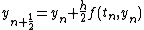
Here, we assume error factor
is constant over the interval . In reality its rate of change is proportional to . Subtracting solutions gives the error estimate: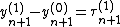
This local error estimate is third order accurate.
The local error estimate can be used to decide how stepsize
should be modified to achieve the desired accuracy. For example, if a local tolerance of is allowed, we could let h evolve like: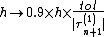
The
is a safety factor to ensure success on the next try. This should, in principle give an error of about in the next try. If , we consider the step successful, and the error estimate is used to improve the solution: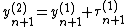
This solution is actually third order accurate in the local scope (second order in the global scope), but since there is no error estimate for it, this doesn't help in reducing the number of steps. This technique is called Richardson extrapolation
Richardson extrapolation
In numerical analysis, Richardson extrapolation is a sequence acceleration method, used to improve the rate of convergence of a sequence. It is named after Lewis Fry Richardson, who introduced the technique in the early 20th century. In the words of Birkhoff and Rota, ".....
.
Beginning with an initial stepsize of
, this theory facilitates our controllable integration of the ODE from point to , using an optimal number of steps given a local error tolerance.Similar methods can be developed for higher order methods, such as the Runge-Kutta 4th order method. Also, a global error tolerance can be achieved by scaling the local error to global scope. However, you might end up with a stepsize that is prohibitively small, especially using this Euler based method.
If you are interested in adaptive stepsize methods that use a so called 'embedded' error estimate, see Fehlberg, Cash-Karp and Dormand-Prince. These methods are considered to be more computationally efficient, but have lower accuracy in their error estimates.