

Gipps' Model
Encyclopedia
Gipps’ Model is a car-following model
named after Peter G. Gipps who developed it in the late-1970s under S.R.C. grants at the Transport Operations Research Group at the University of Newcastle-Upon-Tyne and the Transport Studies Group at the University College London
. It is based directly on driver behavior and expectancy for vehicles in a stream of traffic. Limitations on driver and vehicle parameters for safety purposes mimic the traits of vehicles following vehicles in the front of the traffic stream
. Gipps' Model is differentiated by other models in that Gipps uses a timestep within the function equal to to reduce the computation required for numerical analysis
.
and movement of gases (Lighthill and Whitman (1955) and Richards (1956) postulated the density of traffic to be a function of position; Newell (1955) makes an analogy between vehicle motion along a sparsely populated roadway and the movement of gases). First mention of simulating traffic with “high speed computers” is given by Gerlough and Mathewson (1956) and Goode (1956).
which is defined primarily by one vehicle (noted by subscript n) following another (noted by subscript n-1); reaction time of the following vehicle; the location, speed and acceleration of the following vehicle; and finally, model constants to adjust the model to real-life conditions.
Gipps’ new and improved model should reflect the following properties:
Gipps sets limitations on the model through safety considerations and assuming a driver would estimate his or her speed based on the vehicle in front to be able to come to a full and safe stop if needed (1981). Pipes (1953) and many others have defined following characteristics placed into models based on various driver department codes defining safe following speeds, known informally as a “2 second rule,” though is formally defined through code.
Model Notation
Constraints Leading to Development of Model
Gipps defines the model by a set of limitations. The following vehicle is limited by two constraints: that it will not exceed its driver’s desired speed and its free acceleration should first increase with speed as engine torque increases then decrease to zero as the desired speed is reached.

The third constraint, braking, is given by

for vehicle at point
  , where
  (for vehicle n is given by
 at time
For safety, the driver of vehicle n (the following vehicle) must ensure that the difference between point where vehicle n-1 stops ( ) and the effective size of vehicle n-1 (
 ) is greater than the point where vehicle n stops (
 ). However, Gipps finds the driver of vehicle n allows for an additional buffer and introduces a safety margin, of delay
  when driver n is traveling at speed
  . Thus the braking limitation is given by

Because a driver in traffic cannot estimate , it is replaced by an estimated value
  . Therefore, the above after replacement yields,

If the introduced delay, , is equal to half of the reaction time,
  , and the driver is willing to brake hard, a model system can continue without disruption to flow. Thus, the previous equation can be rewritten with this in mind to yield

If the final assumption is true, that is, the driver travels as fast and safely as possible, the new speed of the driver's vehicle is given by the final equation being Gipps' Model:

where the first argument of the minimization regimes describes an uncongested roadway and headways are large, and the second argument describes congested conditions where headways are small and speeds are limited by followed vehicles.
These two equations used to determine the velocity of a vehicle in the next timestep represent free-flow and congested conditions, respectively. If the vehicle is in free-flow, the free-flow branch of the equation indicates that the speed of the vehicle will increase as a function of its current speed, the speed at which the driver intends to travel, and the acceleration of the vehicle. Analyzing the variables in these two equations, it becomes apparent that as the gap between two vehicles decreases (i.e. a following vehicle approaches a leading vehicle) the velocity given by the congested branch of the equation will decrease and is more likely to prevail.
.
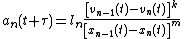
Eulers Method (first order, and perhaps the simplest of the numerical methods) can be used to obtain accurate results, but the timestep would have to be very small, resulting in a greater amount of computation. Also, as a vehicle comes to a stop and the following vehicle approaches it, the term underneath the square root in the congested part of the velocity equation could potentially fall below zero if Euler’s method is being used and the timestep is too large. The position of the vehicle in the next timestep is given by the equation:
x(t+τ)= x(t) +v(t)τ
Higher order methods not only use the velocity in the current timestep, but velocities from the previous timestep to generate a more accurate result. For instance, Huen’s Method (second order) averages the velocity from the current and previous timestep to determine the next position of a vehicle:
Butchers Method (fifth order) uses an even more elegant solution to solve the same problem:
x(t+τ) = x(t) + (1/90)(7k1 + 32k3 + 12k4+ 32k5 + 7k6)τ
k1 = v(t-τ)
k3 = v(t-τ) + (1/4)(v(t) - v(t-τ))
k4 = v(t-τ) + (1/2)(v(t) - v(t-τ))
k5 = v(t-τ) + (3/4)(v(t) - v(t-τ))
k6 = v(t)
Using higher-order methods reduces the probability that the term under the square root in the congested branch of the velocity equation will fall below zero.
For the purpose of simulation, it is important to make sure the velocity and position of every vehicle has been calculated for a timestep before determining the moving along to the next timestep.
In 2000, Wilson used Gipp’s model for simulating driver behavior on a ring road. In this case, every vehicle in the system is following another vehicle – the leader follows the last vehicle. The results of the experiment showed that the cars followed a free-flow time-space trajectory when the density on the ring road was low. However, as the number of vehicles on the road increases (density increases), kinematic waves begin to form as the congested part of the Gipps’ Model velocity equation prevails. An example of a time-space diagram based on Wilson's unstable flow experiment using Gipps' is shown below:
Microscopic traffic flow model
Microscopic traffic flow models are a class of scientific models of vehicular traffic dynamics.In contrast to macroscopic models, microscopic traffic flow models simulate single vehicle-driver units, thus the dynamic variables of the models represent microscopic properties like the position and...
named after Peter G. Gipps who developed it in the late-1970s under S.R.C. grants at the Transport Operations Research Group at the University of Newcastle-Upon-Tyne and the Transport Studies Group at the University College London
University College London
University College London is a public research university located in London, United Kingdom and the oldest and largest constituent college of the federal University of London...
. It is based directly on driver behavior and expectancy for vehicles in a stream of traffic. Limitations on driver and vehicle parameters for safety purposes mimic the traits of vehicles following vehicles in the front of the traffic stream
Traffic flow
Traffic flow, in mathematics and civil engineering, is the study of interactions between vehicles, drivers, and infrastructure , with the aim of understanding and developing an optimal road network with efficient movement of traffic and minimal traffic congestion problems.-History:Attempts to...
. Gipps' Model is differentiated by other models in that Gipps uses a timestep within the function equal to
to reduce the computation required for numerical analysisNumerical analysis
Numerical analysis is the study of algorithms that use numerical approximation for the problems of mathematical analysis ....
.
Introduction
The method of modeling individual cars along a continuous space originates with Chandler et al. (1958), Gazis et al. (1961) , Lee (1966) and Bender and Fenton (1972) , though many other papers proceeded and have since followed. In turn, these papers have bases in several works from the mid-1950s. Of special importance are a few that have analogies to fluid dynamicsFluid dynamics
In physics, fluid dynamics is a sub-discipline of fluid mechanics that deals with fluid flow—the natural science of fluids in motion. It has several subdisciplines itself, including aerodynamics and hydrodynamics...
and movement of gases (Lighthill and Whitman (1955) and Richards (1956) postulated the density of traffic to be a function of position; Newell (1955) makes an analogy between vehicle motion along a sparsely populated roadway and the movement of gases). First mention of simulating traffic with “high speed computers” is given by Gerlough and Mathewson (1956) and Goode (1956).
Model Definition
The impetus for modeling vehicles in a stream of traffic and their subsequent actions and reactions comes from the need to analyze changes to roadway parameters. Indeed, many factors (to include driver, traffic flow and roadway conditions, to name a few) affect how traffic behaves. Gipps (1981) describes models current to that time to be in the general form of:which is defined primarily by one vehicle (noted by subscript n) following another (noted by subscript n-1); reaction time of the following vehicle; the location, speed and acceleration of the following vehicle; and finally, model constants to adjust the model to real-life conditions.
Gipps’ new and improved model should reflect the following properties:
-
- The model should reflect real conditions,
- Model parameters should correspond to observable driver characteristics without undue calculation, and,
- The model should behave as expected when the interval between successive recalculations of speed and position is the same as driver reaction time.
Gipps sets limitations on the model through safety considerations and assuming a driver would estimate his or her speed based on the vehicle in front to be able to come to a full and safe stop if needed (1981). Pipes (1953) and many others have defined following characteristics placed into models based on various driver department codes defining safe following speeds, known informally as a “2 second rule,” though is formally defined through code.
Model Notation
 is the maximum acceleration which the driver of vehicle
  wishes to undertake,
 is the most severe braking that the driver of vehicle
  wishes to undertake
  ,
, is the effective size of vehicle
  , that is, the physical length plus a margin into which the following vehicle is not willing to intrude, even when at rest,
 is the speed at which the driver of vehicle
  wishes to travel,
 is the location of the front of vehicle
  at time *
 ,
, is the speed of vehicle
  at time
  , and
, and is the apparent reaction time, a constant for all vehicles.
Constraints Leading to Development of Model
Gipps defines the model by a set of limitations. The following vehicle is limited by two constraints: that it will not exceed its driver’s desired speed and its free acceleration should first increase with speed as engine torque increases then decrease to zero as the desired speed is reached.
The third constraint, braking, is given by
for vehicle
at point , where (for vehicle n is given by at time For safety, the driver of vehicle n (the following vehicle) must ensure that the difference between point where vehicle n-1 stops (
) and the effective size of vehicle n-1 () is greater than the point where vehicle n stops (). However, Gipps finds the driver of vehicle n allows for an additional buffer and introduces a safety margin, of delay when driver n is traveling at speed . Thus the braking limitation is given byBecause a driver in traffic cannot estimate
, it is replaced by an estimated value . Therefore, the above after replacement yields,If the introduced delay,
, is equal to half of the reaction time, , and the driver is willing to brake hard, a model system can continue without disruption to flow. Thus, the previous equation can be rewritten with this in mind to yieldIf the final assumption is true, that is, the driver travels as fast and safely as possible, the new speed of the driver's vehicle is given by the final equation being Gipps' Model:

where the first argument of the minimization regimes describes an uncongested roadway and headways are large, and the second argument describes congested conditions where headways are small and speeds are limited by followed vehicles.
These two equations used to determine the velocity of a vehicle in the next timestep represent free-flow and congested conditions, respectively. If the vehicle is in free-flow, the free-flow branch of the equation indicates that the speed of the vehicle will increase as a function of its current speed, the speed at which the driver intends to travel, and the acceleration of the vehicle. Analyzing the variables in these two equations, it becomes apparent that as the gap between two vehicles decreases (i.e. a following vehicle approaches a leading vehicle) the velocity given by the congested branch of the equation will decrease and is more likely to prevail.
Using Numerical Methods To Generate Time-Space Diagrams
After determining the velocity of the vehicle at the next timestep, its position at the next timestep should be calculated. There are several numerical (Runge–Kutta) methods that can be used to do this, depending on the accuracy to which the user would prefer. Using higher order methods to calculate a vehicle’s position in the next timestep will yield a result with higher accuracy (if each method uses the same timestep). Numerical methods can also be used to find positions of vehicles in other car following models, such as the intelligent driver modelIntelligent Driver Model
In traffic flow modeling, the intelligent driver model is a time-continuous car-following model for the simulation of freeway and urban traffic...
.
Eulers Method (first order, and perhaps the simplest of the numerical methods) can be used to obtain accurate results, but the timestep would have to be very small, resulting in a greater amount of computation. Also, as a vehicle comes to a stop and the following vehicle approaches it, the term underneath the square root in the congested part of the velocity equation could potentially fall below zero if Euler’s method is being used and the timestep is too large. The position of the vehicle in the next timestep is given by the equation:
x(t+τ)= x(t) +v(t)τ
Higher order methods not only use the velocity in the current timestep, but velocities from the previous timestep to generate a more accurate result. For instance, Huen’s Method (second order) averages the velocity from the current and previous timestep to determine the next position of a vehicle:
Butchers Method (fifth order) uses an even more elegant solution to solve the same problem:
x(t+τ) = x(t) + (1/90)(7k1 + 32k3 + 12k4+ 32k5 + 7k6)τ
k1 = v(t-τ)
k3 = v(t-τ) + (1/4)(v(t) - v(t-τ))
k4 = v(t-τ) + (1/2)(v(t) - v(t-τ))
k5 = v(t-τ) + (3/4)(v(t) - v(t-τ))
k6 = v(t)
Using higher-order methods reduces the probability that the term under the square root in the congested branch of the velocity equation will fall below zero.
For the purpose of simulation, it is important to make sure the velocity and position of every vehicle has been calculated for a timestep before determining the moving along to the next timestep.
In 2000, Wilson used Gipp’s model for simulating driver behavior on a ring road. In this case, every vehicle in the system is following another vehicle – the leader follows the last vehicle. The results of the experiment showed that the cars followed a free-flow time-space trajectory when the density on the ring road was low. However, as the number of vehicles on the road increases (density increases), kinematic waves begin to form as the congested part of the Gipps’ Model velocity equation prevails. An example of a time-space diagram based on Wilson's unstable flow experiment using Gipps' is shown below:
See also
- Intelligent Driver ModelIntelligent Driver ModelIn traffic flow modeling, the intelligent driver model is a time-continuous car-following model for the simulation of freeway and urban traffic...
- List of Runge–Kutta methods
- SimulationSimulationSimulation is the imitation of some real thing available, state of affairs, or process. The act of simulating something generally entails representing certain key characteristics or behaviours of a selected physical or abstract system....
- Traffic SimulationTraffic SimulationTraffic simulation or the simulation of transportation systems is the mathematical modeling of transportation systems through the application of computer software to better help plan, design and operate transportation systems...
Further reading
- Bender, J.C. and Fendon R.E. (1972) On vehicles longitudinal dynamics. In Traffic Flow and Transportation, 19-32. Elsevier, New York.
- Gazis, D.C., Herman R. and Rothery R.W. (1961) Non-linear follow the leader models of traffic flow. Ops. Res. Vol. 9, 545-567.
- Gipps, P.G. (1976) Computer Program MULTSIM for Simulating Output from Vehicle Detectors on a Multi-Lane Signal Controlled Road. Transport Operations Research Group Working Paper No. 20, University of Newcastle-Upon-Tyne.
- Lee, G. (1966) A generalization of linear car-following theory. Ops. Res. Vol. 9, 209-229.
- Seddon, P. A. (1972) Program for simulating the dispersion of platoons in road traffic. Simulation Vol. 18, 81-90.